MT method and PCA use Normal Distribution as background. Sometimes, it could be the difficulty to use these methods.
There is Kernel PCA that use Kernel Method to improve the difficulty.
If we use Kernel PCA to make data of MT method, it is similar to One-Class SVM . Kernel Principal Component MT has similar difficulty of One-Class SVM.
library(kernlab) # Pre-install of "kernlab" is needed
setwd("C:/Rtest")
Data10 <- read.table("Data1.csv", header=T, sep=",")
Data20 <- read.table("Data2.csv", header=T, sep=",")
Data1 <- as.matrix(Data10)
Data2 <- as.matrix(Data20)
pc <- kpca(Data1,kernel="rbfdot", features=10,kpar=list(sigma=0.1)) # Kernel PCMT using 10 principal components
pc1 <- predict(pc, Data1)
pc2 <- predict(pc, Data2)
n <- nrow(pc1)
Ave1 <- colMeans(pc1)
Var1 <- var(pc1)*(n-1)/n
k <- ncol(pc1)
MD1 <- mahalanobis(pc1, Ave1, Var1)/k
MD2 <- mahalanobis(pc2, Ave1, Var1)/k
write.csv(MD1, file = "MD1.csv")
write.csv(MD2, file = "MD2.csv")
R-EDA1 can also use the kernel principal component MT method. You can select four kernel functions.
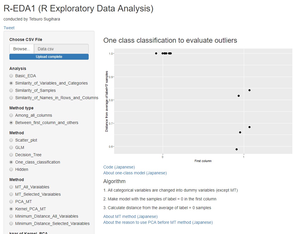
When using kernel principal component analysis, it seems that the graph shown below is often obtained.
The Mahalanobis distance in the unit space (labeled "0" in the graph) is almost 1. In the MT method, the value obtained by dividing the Mahalanobis distance by the number of dimensions is called the "Mahalanobis distance", so it is as expected that the average will be 1. It is good that the average is 1, but the variability is very small.
Another feature of the kernel principal component MT method is that the Mahalanobis distance in the signal space (labeled "1" in the graph) is less than 1 in all samples, depending on how the kernel is selected. Depending on how the parameters are selected, all may be almost 0. In most cases, the value is larger than 1 when the normal MT method is used, but the appearance of the data is reversed.
The author himself has not been able to confirm the mathematical principle of kernel principal component analysis properly, but considering what is happening, if rbfdot is used as the kernel, the training data will be placed on the spherical surface of the multidimensional hypersphere. It seems that a model will be created. Since they are all on a sphere, the distance from the center (average value) of the data seems to be the same and 1.
If you put data with different values ??from the training data for such a model, they seem to be calculated inside the nsphere. If you make a model well, it seems that all the data that deviates from the training data will be calculated so that it is placed at the origin of 0 distance.
If the Mahalanobis distance is close to 1, it is almost the same as the training data, and if it is slightly different, it becomes 0, which may be a convenient property in some cases.

