In Data Science , we often think of the number of variables (the number of columns in table data) and the number of dimensions in the same way. For example, table data with many variables is sometimes called " High dimensional data ".
By the way, in real-life data, at first glance, even if there are many variables, there may be only a few characteristics of variables that need attention in the analysis.
There are two main reasons why "a lot" becomes "a little".
The "effective dimension number" in the title of this page is the number of dimensions that are meaningful in the analysis. Knowing this will give you a better view of your data analysis and reduce your computation time.
"Effective dimension number" is a coined word of the author. If there is already a word with the same meaning in the world, I will replace it, but it seems that there is no such word, so I added it for the time being.
Principal Component Analysis organizes multiple variables into variables called principal components. At this time, if there are 10 original variables, up to 10 principal components can be created, but the characteristics of the data are organized in the order of the first principal component and the second principal component. increase. For example, if there is multicollinearity, the characteristics of the data can be almost expressed up to the third principal component, and the numerical values ??after the fourth principal component are very small. At this time, the number of effective dimensions can be considered to be 3.
There are two ways to determine how many effective dimensions will be, one is to see if the cumulative contribution is close to 1, and the other is to see if the standard deviation of the principal component is very small.
For Feature Engineering , the number of effective dimensions is used when creating a new variable. It is also used for Analysis Using Intermediate Layer .
The number of effective dimensions is an index of how many dimensions a large change in data is represented. In an analysis where small changes are more important, it is not enough to look at the principal components only within the range of effective dimensions.
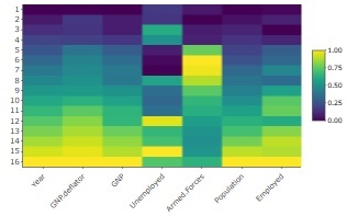
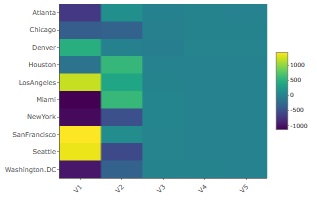
Under Heat Map is, the sample data of R that longley standardization becomes a thing made by. From top to bottom, there are 5 variables with larger values, and there are 2 types and 1 variable with different appearances. Therefore, there are three ways to change.
The result of the principal component analysis of this is as follows. Since the cumulative contribution rate (Cumulative Proportion) exceeds 99% for the third principal component, it matches the result of the heat map of "3 types" above.
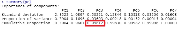
In the case of this example, the number of effective dimensions is considered to be 3.
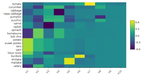
The heat map of the created principal component is below.
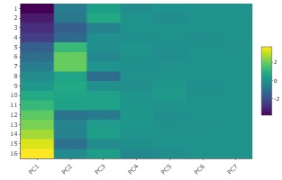
The range of values ??for PC1 is the largest, and it is easy to see the shades up to PC2 and PC3, but it is difficult to see the shades from PC4 to PC7. From this graph, the number of effective dimensions is considered to be 3.
Even if the data in the distance matrix is ??the starting point, there are still valid dimensions. The distance matrix itself represents multiple dimensions in a two-dimensional form, but the data features behind it can be more than three-dimensional.
Using the Multi Dimensional Scaling method , the distance matrix can be converted into coordinate data, but the number of dimensions in which the sample is reasonably placed in the multidimensional space is considered to be the number of effective dimensions.
This method can be used as an AA type analysis method when the data obtained by Evaluation of Pairs is AA type . For data with similarities (closer, larger), it can be used by converting to distance (smaller, closer) data.
For the above longley, the heat map of the result of standardizing, creating a distance matrix, and performing multidimensional scaling with a maximum of 7 dimensions is shown below.
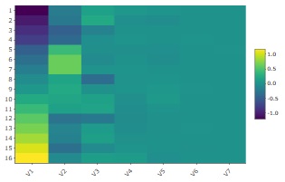
The range of V1 values ??is the largest, and it is easy to see the shades up to V2 and V3, but it is difficult to see the shades from V4 to V7. Therefore, in the case of this example, the number of effective dimensions is considered to be 3.
By the way, this heat map looks very similar to the result of principal component analysis, but the range of color coding is different, for example.
The sample data of R called UScitiesD is the data of the distance matrix between cities in the United States.
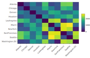
Below is the heat map of the result of multidimensional scaling with up to 5 dimensions .
The shades of V1 and V2 are easy to understand, but V3 to V5 are almost constant values. Therefore, in the case of this example, the number of effective dimensions is considered to be 2. If it is only a city in the United States, it means that the arrangement can be expressed in two dimensions (plane), so the result is in line with the general perception.
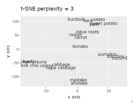
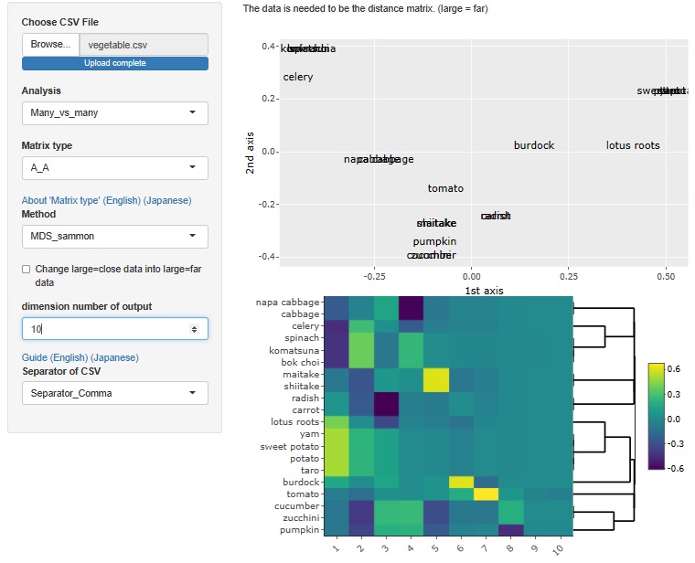
It is the data of the distance matrix made by the author with "similar = 0, dissimilar = 1, uncertain judgment = 0.5" for vegetables. To be precise, if there are samples with a distance of 0, an error will occur in the multidimensional scaling method, so a little random number is added to prevent the distance from becoming exactly 0.
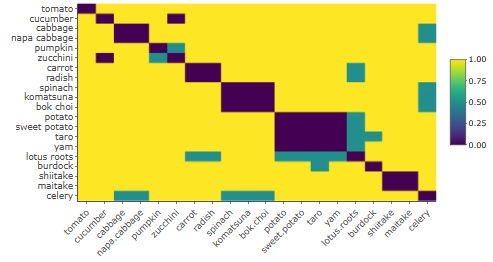
Below is the heatmap of the result of multidimensional scaling with up to 10 dimensions .
Up to V1 and V8, the shade is easy to understand, but V9 and V10 are almost constant values. Therefore, in the case of this example, the number of effective dimensions is considered to be eight. You can see that the author recognizes that there are eight kinds of vegetables when roughly divided.
By the way, if the above distance matrix data is used as the input data of t-SNE , it is arranged so that similar things are gathered on the 2D map, but it is not so clearly divided. Other than the following, the results were similar even if the perplexity was changed. T-SNE is not good with this data.
With R-EDA1 , the above analysis can be performed.
NEXT  Prediction and Simulation
