In the method of making a decision tree , it is common to say "binary tree (also called a binary tree)" and there are always two branches. A relatively easy library to use in R or Python is binary tree.
There is a method called N-try tree (N-branch tree) in the world, and the number of branches can be any number of 2 or more.
In my case, the decision tree is used as a tool for exploring quantitative hypotheses, but it is strict unless it is an N-try tree.
First of all, it is very inconvenient to have to consider the phenomenon in a combination of two divisions according to the result of the decision tree. Even if you can think about it, it is very difficult to get people who do not know the decision tree to understand it in the same way.
Also, in the case of binary trees, the same X often appears in multiple layers, but this makes the relationship between the tree and the mechanism of the phenomenon tight.
It seems that some people think that "a binary tree can express the same thing as an N-try tree in terms of content." Mathematically and logically, even so, it is very inconvenient in practice.
Even if the binary tree method is used, it may be good to have a mechanism to reconstruct the completed tree according to the structure of human cognition.
CHAID is an old method of N-try tree. By the way, I realized that "decision trees are useful!" After I started using CHAID.
CHAID is a mechanism to perform innumerable independence tests (chi-square test).
Therefore, explanatory variables deal with qualitative data. If you want to use quantitative data for the explanatory variables, you can use it by performing one-dimensional clustering and converting it to qualitative data.
* With R CHAID, you need to write the code to convert the quantitative data. IBM's SPSS Modeler contains CHAID, which seems to include the ability to automatically convert quantitative data to qualitative data.
A feature of CHAID is that even if there is a clear difference, it will not branch if the N number is small. This feature is useful because it keeps the branches from becoming finer indiscriminately.
J48 and C4.5 seem to be the same thing.
Explanatory variables can be used both quantitatively and qualitatively. Qualitative data will be N-ary, and quantitative data will be binary, so it is not suitable if you expect N-ary for quantitative data, but unlike CHAID, it is for quantitative data. It is convenient that no preprocessing is required.
Examples of R is in the page, Decision tree by R .
J48 is one of the methods that can be used with Weka. It seems that you can use RWeka in R, but RWeka requires Java settings to be installed. If it's not mandatory to run in R, I think Weka is easier and better.
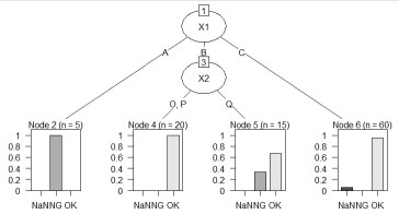
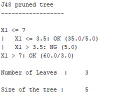
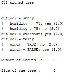
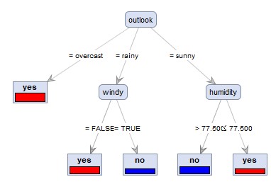
The left is the result of the data created by CHAID "When quantitative data is mixed in X and Y". Quantitative data X1 was chosen and became a binary tree. On the right is the result of the sample data "wether.numeric" in Weka. It became N-try tree.
RapidMiner has a method named "Decision Tree", but since the qualitative data is an N-decimal tree and the quantitative data is a binary tree, it is the same as C4.5 or C4. It seems that it uses an algorithm close to 5.
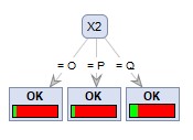
The left is the result of the data created by CHAID "When quantitative data is mixed in X and Y". With the default settings, branching did not occur, and when the parameter "minimal gain" 0.01 was set to 1/10 of the default value, branching occurred.
The right is the result of changing the column name of Y by converting the sample data "wether.numeric" in Weka to csv format. Both became N-try tree.
R-EDA1 is available.
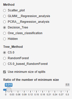
The fineness of the tree when making a decision tree was left to the default, but it can become a huge tree (a tree with fine branches). In the analysis of causality, it is important what happens to the third branch, and huge trees are often unnecessary. Also, if you accept a huge tree, the calculation time can be very long. In addition, huge trees can be called overfitting and are not robust and therefore difficult to use.
Therefore, we have made it possible to set the minimum size of the branch destination. If you check "Use minimum size of splits", you can set it. If you uncheck it, it will be left to the default. For example, if "Ratio of the number of minimum size" is set to "0.1", the minimum branching will be 0.1 for the whole. With 1000 rows of data, it can never be less than 100.
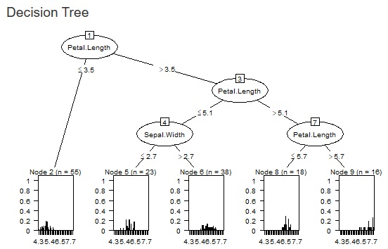
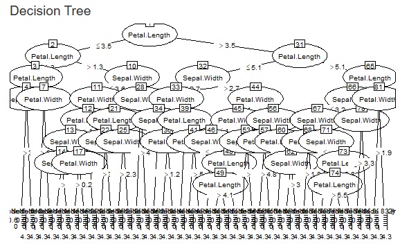
The two figures below are examples when the set values ??are changed for the same data.
 Å@
Å@
NEXT  Random forest
