Decision Tree is a powerful method of data mining . Here, we will introduce how to use it.
The decision tree can also be used for prediction as one of the machine learning methods, but it is not used because it is overfitting or too rough and it is difficult to make it feel just right.
When using a decision tree in R, there are various libraries, and there are advantages and disadvantages.
For practical use, the sample code on this site tries to improve the shortcomings.
rpart is well done, it automatically determines the type of Y and runs a classification tree for qualitative data and a regression tree for quantitative data. Also, X can be used even if qualitative data and quantitative data are mixed.
If you execute it like rpart with CHAID or C5.0 without any special care, an error will occur when "data is logical type or character string type". CHAID and C5.0 have longer code than rpart due to some pre-processing to avoid this error.
Here are some examples of Classification tree and regression tree, and introductory usage.
An example of using R is as follows. (The following is copy-paste and can be used as it is. In this example, it is assumed that the folder named "Rtest" on the C drive contains data with the name "Data.csv" before this code. In addition, it is necessary to install the library "partykit".
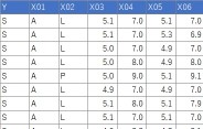
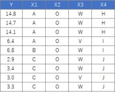
Suppose the data has Y and 20 Xs. There are 90 lines.
setwd("C:/Rtest")
library(partykit)
library(rpart)
Data <- read.csv("Data.csv", header=T)
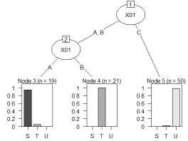
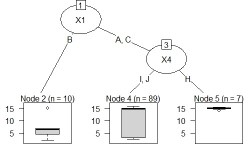
treeModel <- rpart(Y ~ ., data = Data)
plot(as.party(treeModel))
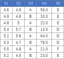
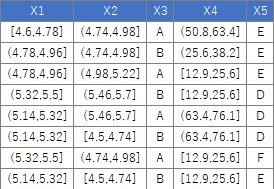
For the following data, the process of "converting the columns of quantitative data into qualitative data" can be performed as follows.
setwd("C:/Rtest")
Data <- read.csv("Data.csv", header=T)
for (i in 1:ncol(Data)) {
if (class(Data[,i]) == "numeric") {
Data[,i] <- droplevels(cut(Data[,i], breaks = 5,include.lowest = TRUE))# When dividing into 5 parts. Quantitative data is converted into qualitative data.
}
}
Suppose the data has Y and four Xs. There are 106 lines.
The code should be exactly the same as above. If Y is quantitative data, it will be treated as a regression tree.
This is an example of N-try tree.
Before this code, you need to install the library "CHAID".
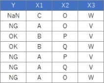
Suppose the data has Y and three Xs. There are 100 lines.
setwd("C:/Rtest")
library(CHAID)
Data <- read.csv("Data.csv", header=T, stringsAsFactors=TRUE)
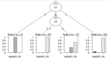
treeModel <- chaid(Y ~ ., data = Data)
plot(treeModel)
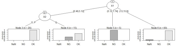
Suppose the data has Y and three Xs. There are 100 lines. X1 is quantitative data.
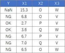
Note that this code can also be used for Y quantitative data.
setwd("C:/Rtest")
library(CHAID)
Data <- read.csv("Data.csv", header=T, stringsAsFactors=TRUE)
for (i in 1:ncol(Data)) {
if (class(Data[,i]) == "numeric") {
Data[,i] <- droplevels(cut(Data[,i], breaks = 5,include.lowest = TRUE))
}
}
treeModel <- chaid(Y ~ ., data = Data)
plot(treeModel)
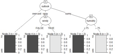
WThe sample data "wether.numeric" in Weka was converted to csv format, and the Y column name was changed, and it did not branch. I think the cause is small data with only 14 rows of this data. Changing the parameters may change the situation, but I haven't tried that much.
C5.0 is a method that can be used even if quantitative and qualitative data are mixed. Quantitative data is binary and qualitative data is N-ary.
It can be used in R's C50 library. Installation is easy. In the code below, first, when reading the csv file, the columns that are automatically recognized as string type (strings) are converted to factor type (factor). The 5 rows starting with for convert the columns that are automatically recognized as logical to factor type. Failure to do these pre-processing will result in an error in the C50 package.
setwd("C:/Rtest")
library(C50)
library(partykit)
Data <- read.csv("Data.csv", header=T, stringsAsFactors=TRUE)
if (class(Data$Y) == "numeric") {
Data$Y <- droplevels(cut(Data$Y, breaks = 5,include.lowest = TRUE))
}
for (i in 1:ncol(Data)) {
if (class(Data[,i]) == "logical") {
Data[,i] <- as.factor(Data[,i])
}
}
treeModel <- C5.0(Y ~ ., data = Data)
plot(as.party(treeModel))
The left is the result of the data created by CHAID "When quantitative data is mixed in X and Y". The right is the result of changing the column name of Y by converting the sample data "wether.numeric" in Weka to csv format. The result is almost the same as Weka's J48.

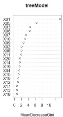
This is an example of a Random forest.
Before this code, you need to install the library "randomForst".
Suppose the data has Y and 20 Xs. There are 90 lines.
setwd("C:/Rtest")
library(randomForest)
Data <- read.csv("Data.csv", header=T, stringsAsFactors=TRUE)
treeModel <- randomForest(Y ~ ., data = Data, ntree = 10)
varImpPlot(treeModel)
The method of obtaining the predicted value is the same as other methods in how to use the Software for Prediction.
The randomForest library is built to help you find and predict important variables using Random Forest . However, it seems that there is no function to output the individual trees (forests) that are created in the middle of those calculations, although you can see such information.
So, I made a code to output the structure of the tree.
It's based on rpart, CAHID, and C5.0, not the randomForest code. Since a typical random forest is a binary tree, it is based on rpart that the result is close to that of a tree in the middle of a general random forest calculation. I wanted something from N-tri , so I also made CHAID-based and C5.0-based random forests.
The point is how to create a dataset for 10 times. With this code, it's convenient to be able to adjust it yourself.
Suppose the data has Y and 20 Xs. There are 90 lines.
setwd("C:/Rtest")
library(rpart)
library(partykit)
Data <- read.csv("Data.csv", header=T)
ncolMax <- ncol(Data)
nrowMax <- nrow(Data)
DataY <- Data$Y
Data$Y <- NULL
for (i in 1:9) {
DataX <- Data[,runif (floor(sqrt(ncolMax)), max=ncolMax)]
Data1 <- transform(DataX, Y = DataY)Å@
Data2 <- Data1[runif (floor(sqrt(nrowMax)), ,max=nrowMax), ]# Randomly select the number of rows with the square root of the number of rows
treeModel <- rpart(Y ~ ., data = Data2, minsplit = 3)
jpeg(paste("plot",i,".jpg"), width = 300, height = 300)
plot(as.party(treeModel))
dev.off()
}
Running this code will create as many resulting image files as there are trees in your working directory.
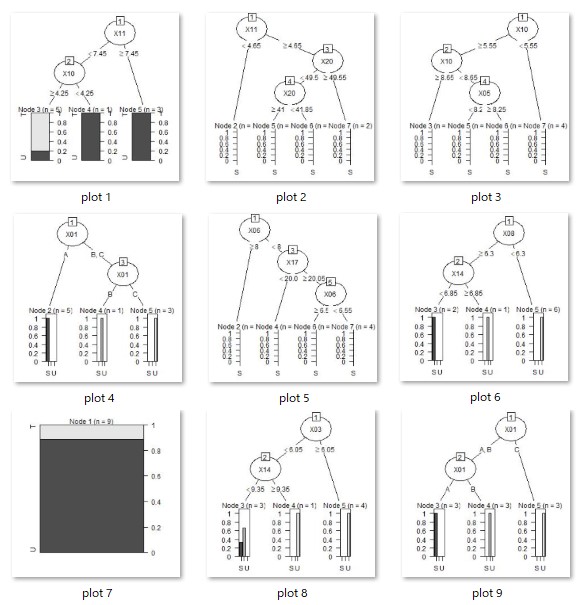
As intended, we have also created a tree with three or more branches.
setwd("C:/Rtest")
library(C50)
library(partykit)
Data <- read.csv("Data.csv", header=T, stringsAsFactors=TRUE)
ncolMax <- ncol(Data)
nrowMax <- nrow(Data)
if (class(Data$Y) == "numeric") {
Data$Y <- droplevels(cut(Data$Y, breaks = 5,include.lowest = TRUE))
}
DataY <- Data$Yv
for (i in 1:ncolMax) {
if (class(Data[,i]) == "logical") {
Data[,i] <- as.factor(Data[,i])
}
}
Data$Y <- NULL
for (i in 1:9) {
DataX <- Data[,runif (floor(sqrt(ncolMax)), max=ncolMax)]
Data1 <- transform(DataX, Y = DataY)Å@
Data2 <- Data1[runif (floor(sqrt(nrowMax)), ,max=nrowMax), ]
treeModel <- C5.0(Y ~ ., data = Data2)
jpeg(paste("plot",i,".jpg"), width = 300, height = 300)
plot(as.party(treeModel))
dev.off()
}
Running this code will create as many resulting image files as there are trees in your working directory.
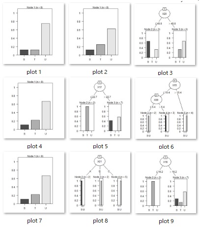
As intended, we have also created a tree with three or more branches.
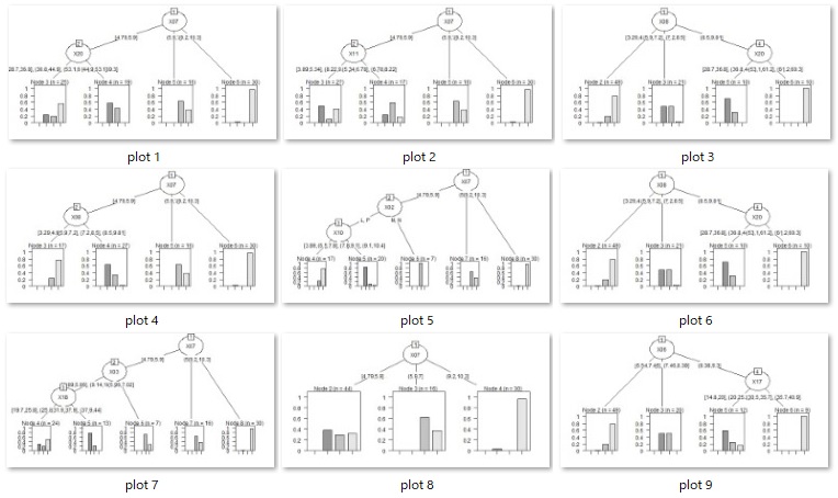
The feature of the code below is that, in addition to being CHAID, it is the "column bagging" written on the ensemble learning page. That is, sampling is only columns, not rows.
It takes longer to calculate than the C5.0 based one.
setwd("C:/Rtest")
library(CHAID)
Data <- read.csv("Data.csv", header=T, stringsAsFactors=TRUE)
ncolMax <- ncol(Data)
nrowMax <- nrow(Data)
for (i in 1:ncolMax) {
if (class(Data[,i]) == "numeric") {
Data[,i] <- droplevels(cut(Data[,i], breaks = 5,include.lowest = TRUE))
}
}
DataY <- Data$Y
Data$Y <- NULL
for (i in 1:9) {
DataX <- Data[,runif (floor(sqrt(ncolMax)), max=ncolMax)]
Data1 <- transform(DataX, Y = DataY)Å@
#Data2 <- Data1[runif (floor(sqrt(nrowMax)), ,max=nrowMax), ]
Data2 <- Data1
treeModel <- chaid(Y ~ ., data = Data2)
jpeg(paste("plot",i,".jpg"), width = 600, height = 300)
plot(treeModel)
dev.off()
}
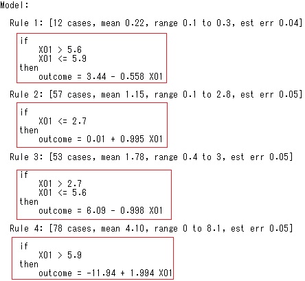
Example of Model tree.
setwd("C:/Rtest")
library(Cubist)
library(ggplot2)
Data <- read.csv("Data.csv", header=T)
Ydata <- Data$Y
Data$Y<-NULL
Cu <- cubist(y = Ydata, x=Data, data = Data)
summary(Cu)
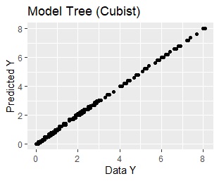
Output <- predict(Cu,Data)
Data2 <- cbind(Data, Output)
ggplot(Data2, aes(x=Y, y=Output)) + geom_point()+xlab("Data Y")+ylab("Predicted Y")+ggtitle("Model Tree (Cubist)")
Examples to limit the number of rules as 3
Cu <- cubist(y = Ydata, x=Data, data = Data, control=cubistControl(rules = 3))
