The word "distance" is used in everyday life. Mahalanobis' Distance (MD) is, as the name suggests, a type of distance.
The MT method is a representative one that uses the Mahalanobis distance. The M comes from where we use the Mahalanobis distance. Otherwise, for example, Discriminant Analysis also uses the Mahalanobis distance.
In everyday life, when we talk about "distance", we often refer to Euclidean distance.
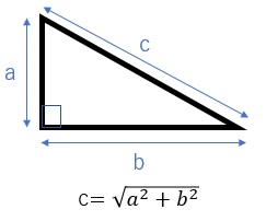
The Euclidean distance is basically the same as the length of the hypotenuse of a right triangle.
The calculation method of Mahalanobis distance is quite different from this one, but I think it is easier to understand "What is Mahalanobis distance?" by starting with Euclidean distance and comparison.
In daily life, when we talk about distance, we use the term "distance between point A and point B". It is used interchangeably with "length".
Both Mahalanobis distance and Euclidean distance are labeled as "distance", but they can also be used for things that are not "length". In Data Science , distance is sometimes used as an indicator of "A and B are similar".
Mahalanobis distance and Euclidean distance are equal when calculated with data where the diagonal elements of the covariance matrix are 1 and the others are 0.
If the diagonal elements of the covariance matrix are 1 and the others are 0, then the standard deviation of each variable is 1 and there is no correlation between the variables. If the completely unrelated items are variables and the data is standardized , then this case is closer.
The Euclidean distance can be obtained by the square root of the sum of the squared numbers, but the Mahalanobis distance requires matrix calculation and variance calculation, so the calculation is complicated.
When there is a correlation between variables, Mahalanobis distance takes it into account in the calculation. Euclidean distance is not considered.
In situations where Euclidean distance is used, for example, there are X and Y directions, but in everyday distances, these can be considered independent, so there is no particular problem in that correlation is not considered.
Since the Mahalanobis distance takes correlation into account, it can be used as an index that considers "similar properties" when there are similar properties between variables.
In Euclidean distance, if the original coordinates were in meters, the distance units would also be in meters. The distance has units.
In Mahalanobis distance definition 1 (described later), the average value of the distance is the "number of variables" for variables of any unit. In definitions 2 and 3 (described later), the average value of the distance is "1" regardless of the unit variable.
As you can see from this, the Mahalanobis distance is dimensionless (does not have units).
The Euclidean distance has a specific unit, so you can use it as you imagine in a real story. On the other hand, the Mahalanobis distance cannot be used in such a way.
Mahalanobis distance can be used as a meaningful index even if variables with different units such as meters and kilograms are mixed. This advantage is a good thing about nondimensionalization.
On the other hand, calculating the Euclidean distance for data that contains variables with different units is a calculation like "square of meters + square of kilograms", so from the point of view of Dimension Analysis , it is a calculation that should not be done. is.
By the way, if you calculate the Euclidean distance without worrying about units, the absolute value of the number is a great indicator of a large variable. For example, if you have two variables, kilograms and meters, and if you convert the kilogram variable to grams, the calculated Euclidean distance will be different. In grams, the effect of the weight variable appears more strongly on the Euclidean distance.
When using the Euclidean distance because it is easy to calculate or considers the variables to be uncorrelated, it is recommended to preprocess the data using Standardization , Normalization , Principal Component Analysis , etc. Is good. However, this usage makes the distance dimensionless, so one of the advantages of using the Euclidean distance is lost.
There are several definitions of "Mahalanobis distance" in the world. It differs between mathematics (statistics) and Quality Engineering( MT method ), so be careful when using it.
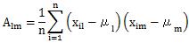
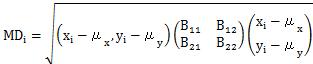
Let's take the case of two variables, x and y, as an example.
"i" means "ith data".

In the MT method , the division by the number of variables (k) is added to the calculation formula of Definition 1.
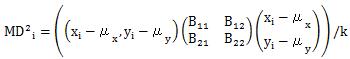
The above is a formula for calculating the " square of Mahalanobis distance", but in practice using the MT method, " square of Mahalanobis distance" is abbreviated as "Mahalanobis distance". There are many
The average value of the square of the Mahalanobis distance below is also the same, but in situations where the Mahalanobis distance is actually used or discussed, the squared value before the square root is better for data analysis. I can do it.
Definition 3 has the same MD numbers as Definition 2, but is a convenient method when you want to analyze the data in detail.
After standardizing the data, calculate Definition 2.
One caveat, the standard deviation used in standardization is the sample standard deviation obtained by dividing the denominator by n. When standardizing in practice, dividing by n or dividing by n-1 often does not change the conclusion, but when calculating the Mahalanobis distance, you need to be careful about which one to use. The calculation of the average value may not match.
There are two main reasons why the Mahalanobis distance calculation does not go well, as in the case when the calculation is wrong with the MT method . If you proceed with the calculation with Definition 3, it will be easier to find out which reason is when things go wrong.
First, the standard deviation of each variable is calculated, so it is convenient to use this value to check whether there are variables with a standard deviation of 0, that is, variables that contain only the same value. If you try to calculate the Mahalanobis distance with such variables included, you will get an error. Also
, the covariance matrix obtained from the standardized values ??is the correlation matrix, and the matrix elements are the correlation coefficients . A correlation matrix is??useful for checking multicollinearity . The Mahalanobis distance calculation gives an error when there are combinations of variables with multicollinearity .
There is an Excel sample file in the MT method procedure , which uses definition 3.
In calculating the Mahalanobis distance, we use the mean and the variance of all the samples we prepared. Because of this treatment, the calculated average Mahalanobis distance for each sample has a characteristic. This feature can be exploited in data analysis.
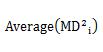
For definition 1, the average squared Mahalanobis distance is exactly the same as the number of variables . That is
In the above example, there are two variables, x and y, so k is 2.
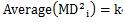
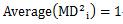
In the case of definitions 2 and 3, it is 1 regardless of the number of variables. , that is
 <
<
If you know what the theoretical average value will be, you can check whether the Mahalanobis distance calculation is correct or not, and it will be an index when analyzing the value.
When you actually use the Mahalanobis distance, you may analyze it by changing the combination of variables used in the calculation.
In the case of definition 1, when the Mahalanobis distance is calculated as "2.4", if the number of variables is 3, it is "smaller than the average value", and if the number of variables is 2, it is "larger than the average value", the way of thinking will change.
In the case of definitions 2 and 3, the average value of the squared Mahalanobis distance is always 1, regardless of the number of variables. Therefore, without worrying about the number of variables, you can always consider 1 as a guideline. It is useful when judging abnormalities by the MT method .
It is strange that the average value of the squared Mahalanobis distance is a perfect integer.
Let's check the case of definition 2.

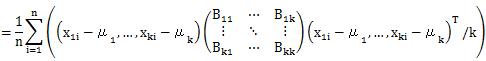
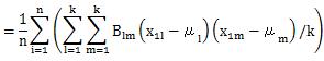
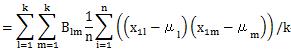
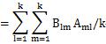
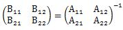
The formula that appears here is the same formula as the diagonal elements of the matrix of the product of B and A. The matrix of the product of B and A is an identity matrix, so its diagonal is 1. We will use this in the next transformation.


Again, when calculating the covariance and standard deviation, if the denominator is not "n", the above formula will not be expanded.
NEXT  Difference between MT method and Hotering theory
