For quasi-periodic type sensor data among Factory sensor data, it is as follows Quasi-periodic Data Analysis. Use variables that tell you the beginning and end of the cycle, We read the similarities between the beginning and the end from the graph and create those variables before using them.
With flow-type sensor data, this information is not available, so it is not possible to create Type 3 data in the same way. So we take a different approach.
This page is sensor data that the causative system accumulates every 1 minute, etc. It is assumed that the result system has time information such as each product or each event occurrence.
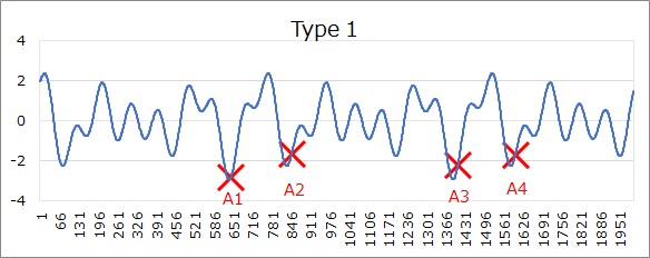
In the image above, the X indicates when the event occurred.
In this example, the graph shows that the event occurred a little after the value dropped significantly and then started to rise. With this volume of data, it may be okay to draw conclusions with such considerations, If the amount is large and it is difficult to judge based on the appearance of the graph, there are the following aggregation methods.
The flow type uses Time Difference of Cause-Effect.
When there is data for the result system, if there is data for the causal system related to it, the time is before the result system. The end of the data to be cut uses this knowledge.
With the flow type, the beginning of the data to be cut is not easily determined. It all begins, "Considering the speed of the flow, there is a causal relationship at most for this amount of time." "Until the total value (integral) reaches this value", It is necessary to decide by considering "until a certain value is found first".
When creating Type 2 data from actual flow-type data, the data is extracted from the most recent time in a form that goes back to the past. When it finds the same time as the result data, it will flag it and cut out the determined range from there.
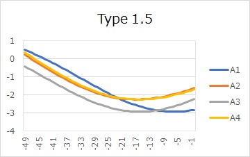
In the example below, 50 pieces of data are extracted from the timing of the event in retrospect. This summarization method is equivalent to the analysis of Type 1.5 data in the case of quasi-periodic data. At this point, the following steps are the same as Quasi-periodic Data Analysis.
Since the direction of time when exploring data is opposite to that of the quasi-periodic type, this site calls it reverse time aggregation. Although the source used to cut data and the direction of time to search are different, the basic procedure for creating secondary data is the same as for the quasi-periodic type.
In reverse time aggregation, the time of the result system data is used to aggregate, so Type 3 data can be created as well as type 2 data.
On the Time Difference of Cause-Effecte, there is a story that it is not easy to link when analyzing cause and effect, but reverse time aggregation is a countermeasure.
Passing Analysis looks at changes in the temporal effects of what happened as a cause. The time of the cause is clear.
Analysis using inverse time aggregation looks at the evolution of what happened as a result from the past. The time of the result is clear.
NEXT  Self Correlation Analysis
