Top Page | Upper Page | Contents | About This Site | JAPANESE

Principal Component MT

The idea of Aprroach for Chance of MT is important. But there is the case that we make the MT model quickly.

In this case, Principal Component Analysis (PCA) is good to make data for MT method .

As Logic to Use "Number of Variance > Number of Samples"

In MT method , the data of Unit Space must be
"Number of Variance < Number of Samples"
to calculate MD.

But we can change
"Number of Variance > Number of Samples"
into
"Number of Variance < Number of Samples"
by PCA.

Principal Component MT by R

Code

Emapmle of R is below

setwd("C:/Rtest")
Data1 <- read.table("Data1.csv", header=T, sep=",") # Input unit space data
Data2 <- read.table("Data2.csv", header=T, sep=",") # Input signal space data
pc <- prcomp(Data1, scale=TRUE) # PCA of unit space data
summary(pc) # Cumulative Proportion is the information to deceide the number of principal component.
pc1 <- predict(pc, Data1)[,1:3] # 3 principal components are used
pc2 <- predict(pc, Data2)[,1:3]
n <- nrow(pc1)
Ave1 <- colMeans(pc1)
Var1 <- var(pc1)*(n-1)/n
k <- ncol(pc1)
MD1 <- mahalanobis(pc1, Ave1, Var1)/k
MD2 <- mahalanobis(pc2, Ave1, Var1)/k
write.csv(MD1, file = "MD1.csv")
write.csv(MD2, file = "MD2.csv")

R-EDA1

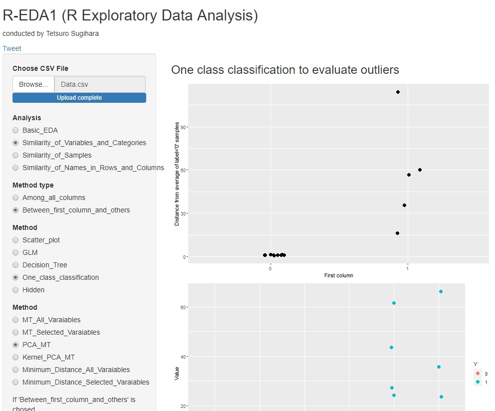
With R-EDA1 , the main component MT method can be used.

The sum of squares of standardized principal component scores can also take advantage of the property of matching the sum of squares of Mahalanobis distances. A graph is also created in which the square of the standardized principal component score is calculated for each principal component, so you can see which principal component affects the difference in labels.

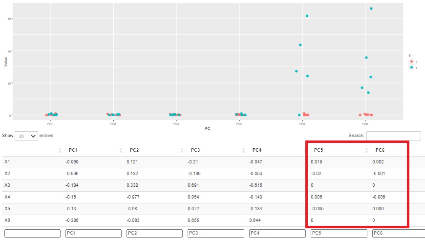
Also, since the correlation coefficient between the principal component and the original variable is known, the relationship with the original variable can be investigated. In the example below, you can see that the two main components, PC5 and PC6, influence the difference between normal and abnormal.

Furthermore, in this example, we can see that PC5 and PC6 are poorly correlated with any variable in the original data. In other words, you can see that what is different from what you normally see in the original data affects normal and abnormal.

NEXT Kernel Principal Component MT