
is an expression that represents a straight line with a slope of A and an intercept of B.
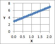
is an expression that represents a straight line with a slope of A and an intercept of B.
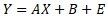
is a model for regression analysis. E is the error, and the presence of this part expresses that the data is arranged in a form close to a straight line while variing. On this site, we call it the variability model.
The above equation is a type of additive model. Although not as famous as the additive model, there is also a multiplication model that includes errors. This page is about a multiplicative model with errors.
There are two main types of explanations in the world about factorial models that include errors. The shape of the error term is different.
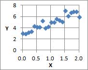
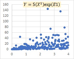
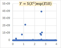
On this page, we refer to the "multiplicative model exp(E)" as the following equation.
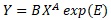
As you can see on Additive model and multiplicative model page, this equation is obtained when the additive model is transformed.
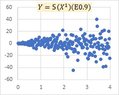
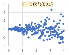
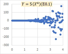
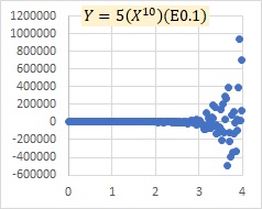
On this page, we refer to the equation "multiplicative model E" as follows.

As a multiplication, it has a straightforward form.
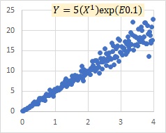
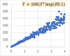
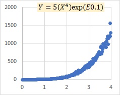
"E0.1" in the graph indicates that the number in parentheses is a normally distributed random number with a mean value of 0 and a standard deviation of 0.1.
This is an example of the multiplicative model exp(E). It is similar to the multiplicative model E in that it represents that as X increases, the variation of Y increases, but it also represents that Y becomes larger overall.
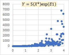
This is an example of a multiplicative model E. The model shows that as X grows, the variation of Y, both positive and negative, increases.
In the graph above, there is no periodicity. If you want to deal with periodicity, it is easier to deal with it with additive models, such as AR Model and Others.
If you look up "multiplicative model", you will find many articles that introduce it as a method of time series analysis.
If we think of X as a time series, the multiplicative model is a model that expresses that the influence of uncertainties increases as time passes.
Additive and multiplicative models look quite different, but they have a relationship that can be transformed. It is summarized on Additive model and multiplicative model page.
Additive model and Proportional variance are similar, but they are used in very different ways.
Above, I have written an example of two types of multiplicative models, where the mean value is 0. In regression analysis, there is a variation between the top and bottom of the regression line, and the regression line represents the average value of the variation. I think it's a natural way of thinking to say that E "varies so that the average value is 0".
By the way, if you start thinking that "error is such a property...", you will be told that the average value is 0. If you don't care about what it is in reality, but only think about the form of the equation of the multiplicative model, you can create an expression other than 0.
On this site, when the average value is 0, it is called "narrow", and everything else is called "broad".
In a broad sense, various forms can be considered, but if we assume "for example, a normal distribution with a mean value of 5", The multiplicative model has the properties of an additive model. These properties are summarized in the page Additive model like multiplicative model.
In the narrow multiplicative model, the effect of variation is included in the "E" part. In this model, the "E" is included with the idea that "I don't know what it is, but there is a variation, and the magnitude of the variation can be expressed by E."
In a broad multiplicative model, E is something that has a variable property. Y is thought of as a combination of other elements on such a thing.
On this page, the multiplicative model is divided into narrow and broad based on the shape of the expression, but the physical meaning that can be included in it is not the difference between "narrow and wide".
NEXT  Additive model and multiplicative model
