Quantification type III is a type of quantification theory . It is known to be mathematically the same as correspondence analysis , although the form of the data used as an example is different . As you can see on the correspondence analysis page, correspondence analysis and principal component analysis are very similar, so quantification type III is also a very similar method to principal component analysis.
The value of the ranking data when this state is created is interpreted as a meaningful order for each category.
In the original quantification type III, row and column sorting is performed by a mathematical procedure.
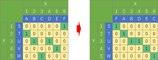
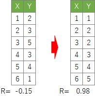
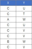
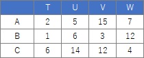
Suppose the original data is matrix data like the one on the left. In Quantification Class III, the matrix is ??rearranged so that the part with "1" is lined up diagonally as much as possible. Then, the correlation coefficient between the X and Y rank data of the part with "1" is maximized.
The value of the ranking data when this state is created is interpreted as a meaningful order for each category.
In the original quantification type III, row and column sorting is performed by a mathematical procedure.
First, you'll see some meaningful order for each of the X and Y categories. In this sense, the categories are "quantified".
Then you'll also see how to correlate for each of the X and Y categories.
On this site, I thought about "quantification III in a broad sense".
The target data are Data1, 2, and 4 of how to divide the pages of quantification theory .
We also think that there is no objective variable. An analysis method for obtaining coordinate data of two types of categories. Not only the original quantification type III, but also principal component analysis and correspondence analysis are included.
Principal component analysis is the main focus of Quantification III in a broad sense . When it comes to quantification type III in a broad sense, it also deals with data that is a mixture of qualitative and quantitative variables, but correspondence analysis is not a theory that deals with such data.
Principal component analysis can be used to analyze variable grouping and sample grouping .
On the other hand, Quantification III in a broad sense can be used for analysis of grouping of individual categories and analysis of grouping of samples .
When using principal component analysis for quantification type III in a broad sense, it is the principal component analysis itself except for the part that creates input data. However, by creating dummy-transformed data, the original qualitative variables are not analyzed for variable grouping, but for individual category grouping .
On the association analysis page, I write an example of converting quantitative variables into qualitative variables for data that is a mixture of qualitative variables and quantitative variables. For data with a mixture of quantitative and qualitative variables , I think the best approach is to "look at the structure of the data" using this method or using multiple correspondence analysis .
Although it is possible to perform principal component analysis by performing dummy conversion on qualitative variables , the correlation coefficient between variables created by dummy conversion and quantitative variables tends to be very low. The relationship between variables that were originally quantitative variables, the relationship between variables that were originally quantitative variables and the quantitative variables created by dummy conversion, and the three types of combinations of quantitative variables created by dummy conversion are different. I have to handle it, but once I do dummy conversion, I can not handle it differently, so I can not evaluate the relationship of variables well.
Therefore, for data that is a mixture of qualitative and quantitative variables, I think it is best to bring it into the analysis method for qualitative variables.
If there is only one quantitative variable, you can use it as the objective variable and use quantification type I in a broad sense or a regression tree to see the structure of the data.
There are some interesting qualities when starting with Data 1 and 4.
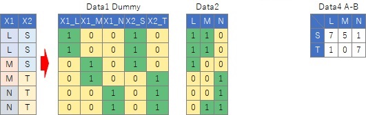
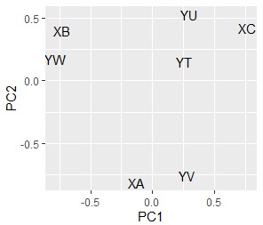
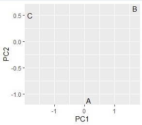
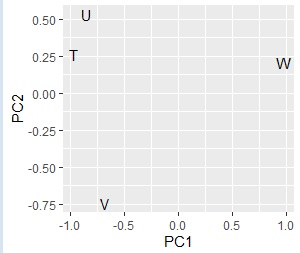
The two graphs below start with the same data and have different analysis methods. On the left is a graph that combines the principal component scores and factor loadings by dividing the data into a contingency table and then performing principal component analysis. The right is a graph of factor loading when principal component analysis is performed after dummy conversion of data .
Although there is a difference in symmetry, almost the same graph is made.
Even if you do not have the original data to create a contingency table, you can get almost the same results as when you analyzed the original data, so you can see that you can perform the same analysis as when you have the original data without the original data. ..
The method of using a contingency table targets a contingency table, so it cannot be used when there are three or more original qualitative variables (three columns). The method of using the dummy transformation can be done with any number of original qualitative variables.
Also, the method using the dummy conversion in the graph above does not include the result of the principal component score. You can also analyze the grouping of samples from the principal component score information .
In this example, it is assumed that the folder named "Rtest" on the C drive contains data with the name "Data.csv".
setwd ("C: / Rtest") #Change working directory
Data <-read.csv ("Data.csv", header = T) #Read data
crs < -table (Data $ X, Data $ Y) #
Create a scatter table pc <-prcomp (crs, scale = TRUE) # Principal component analysis
pc1 <-pc $ x # Get principal component score
pc1 <-transform (pc1, name = rownames (pc1)) # Add row name
library (ggplot2) #Load package
ggplot (pc1, aes (x = PC1, y = PC2, label = name)) + geom_text () # Scatter plot of words with 1st and 2nd principal components
# Up to this point, it was a grouping of categories on the X side. After this is the grouping of categories on the Y side.
pc2 <-sweep (pc $ rotation, MARGIN = 2, pc $ sdev, FUN = "*") # Calculate factor load
pc2 <-transform ( pc2, name = rownames (pc2)) # Rewrite name
ggplot ( pc2, aes (x = PC1, y = PC2, label = name)) + geom_text () # Scatter plot of words
# Combine the two results.
pc3 <-rbind (pc1, pc2) # Combine two results
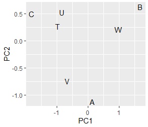
ggplot (pc3, aes (x = PC1, y = PC2, label = name)) + geom_text () # Scatter plot of words Comparing the
contingency table and the graph , You can see that the relationships where the numbers are large are located close together.
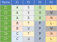
The sample data uses the following. It works even if there is no "Name" column.
library (dummies) # Load library
setwd ("C: / Rtest") # Change working directory
Data <-read.csv ("Data.csv", header = T) # Read data
DataName <-Data $ Name # Store Name column with a different name
Data $ Name <-NULL # Remove Name column from data and leave only X column Data_dmy <-dummy.data.frame (Data) # Dummy conversion
pc <-prcomp ( Data_dmy, scale = TRUE) # Principal component analysis
summary (pc) # "Cumulative Proportion" is the cumulative contribution rate.
pc1 <-pc $ x # Get the principal component score
pc1 <-transform (pc1, name = DataName) # Add sample name
pc1 $ Index <-row.names (Data) # Create a column named Index and the contents are Make it a line number
library (ggplot2) #Load package
ggplot (pc1, aes (x = PC1, y = PC2, label = name)) + geom_text () # Scatter plot of words with 1st and 2nd principal components
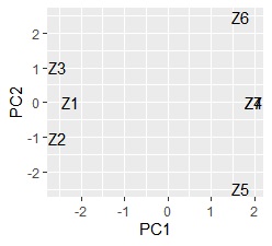
Z4 and Z7 overlap. Since quantification type III is based on principal component analysis , samples may be allocated in three or more dimensions when the sample grouping is analyzed , and it cannot be seen well in the scatter plot. If you want to see it in two dimensions, the multidimensional scaling method is better.
pc2 <-sweep (pc $ rotation, MARGIN = 2, pc $ sdev, FUN = "*") # Calculate factor load
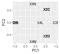
pc2 <-transform (pc2, nameCol = rownames (pc2)) # Scatter plot of words
ggplot ( pc2, aes (x = PC1, y = PC2, label = nameCol)) + geom_text () # Scatter plot of words
NEXT  Text Mining
