Of the many-to-many analyzes , there are quite a few mathematics and graphs for AA type analysis .
On the other hand, AB-type analysis of the For, mathematical While it seems there are, graph, simultaneous edge view and a bipartite graph there is only, in these just might be little time that was analyzed by mathematical. This page is the solution for graphing the results of correspondence analysis .
You can't find the article easily by searching "Tripartite graph", but you can find various articles by searching "Tripartite graph". "Multidimensional simultaneous attachment map" is the name given by the author. As far as I investigated, there seemed to be no same projection in the world.
The original data when drawing the simultaneous attachment diagram is as shown on the left side of the diagram below. By a mathematical method, C that connects A and B is found and it is on the right side, but since only two of C can be used for simultaneous attachment (scatter plot), only two are seen from the left. Seems to be common.
If you know that there are 3 or more Cs, you will be worried about overlooking the analysis, and you will have to make various combinations of Cs at the same time, but if you can make a lot of graphs, it will be a comprehensive judgment. Will be difficult.
By the way, what I see in the analysis using the simultaneous attachment diagram is "Which of the elements A and B is closer?", And I am concerned about "What about C?" It may not be.
The multidimensional simultaneous attachment diagram is a method of condensing up to two elements of C, which have three or more elements, by specializing in "it is only necessary to know which of the elements A and B is close to each other!" .. For this condensation, the high dimension is compressed into two dimensions and the visualization method is used.
By using a bipartite graph, you can directly see the relationship between ABO data as a network graph.
The data used for simultaneous attachment is data in which the elements of A and the elements of A and B are not connected, but the elements of A and C and the elements of B and C are connected. You can create a network graph by creating an adjacency matrix of all the elements A, B, and C, but it's easier to take advantage of this property of the data and tweak the bipartite graph a bit.
A bipartite graph is a way to see the relationship between A, B, and C. In the multidimensional simultaneous attachment diagram, C, which is multidimensional, is compressed into two dimensions to take measures, but in the three-part graph, the number of dimensions remains, so the relationship with C can also be seen.
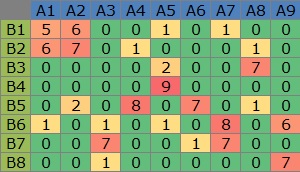
In this example, it is assumed that the folder named "Rtest" on the C drive contains the data that is a contingency table with the name "Data.csv".
library (MASS) # Load package
setwd ("C: / Rtest") # Change working directory
Data <-read.csv ("Data.csv", header = T, row.names = 1) # Read data
pc <- Corresp (Data, nf = min (ncol (Data), nrow (Data))) # correspondence analysis
pc1 <- pc $ Cscore # reading scores
pc1 <- transform (pc1, name1 = rownames (pc1), name2 = "A") # Add row name
pc2 <-pc $ rscore # Read score
pc2 < -transform (pc2, name1 = rownames (pc2), name2 = "B") # Add column name
Data1 <-rbind ( pc1, pc2) # Combine data
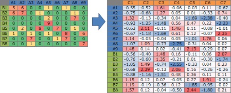
round (pc $ cor ^ 2 / sum (pc $ cor ^ 2), 2) # Find the contribution rate.

The data "Data1" is as below. This will be used for subsequent graph creation.
I'm using multidimensional scaling here, but depending on the data , other methods of compressing and visualizing higher dimensions to 2D may be better.
In the above example, the 6th and subsequent eigenvalues ??have a low contribution rate, so we will exclude them from the analysis. By the way, if you put a part with a low contribution rate, it seems to be noise and it can not be separated cleanly.
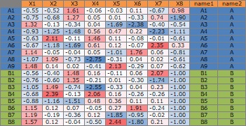
MaxN = 5 #Specify the number of eigenvalues ??to use Data11 <-Data1 [, 1: MaxN] #Specify a column with items Data11_dist < -dist (Data11) #Calculate the distance between samples sn <-sammon (Data11_dist) # Multidimensional scaling output <-sn $ points # Extraction of the obtained 2D data Data2 <-cbind (output, Data1) # Combine theÅ@ original data with the results of the multidimensional scaling. library (ggplot2) #Load package # ggplot (Data2, aes (x = Data2 [, 1], y = Data2 [, 2], label = name1)) + geom_text (aes (colour = name2)) # Use Name Scatter plot of the words
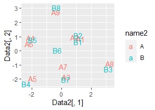
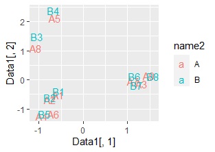
I was able to create the simultaneous attachment plot as I expected.
By the way, if you perform correspondence analysis and normally make a simultaneous attachment diagram with the first and second variables, it will be as follows.
MaxN = 5 # specifies the number of eigenvalues to use
library (igraph) # reads package
library (sigmoid) # reads package
data1p = Data1 [, 1: MaxN] # extracted analyte data
names (Data1p) = paste ( names (Data1p), "+", sep = "")
#Rename column DM.matp = apply (Data1p, c (1,2), relu) # Convert the following values ??to 0
Data1m = -Data1 [ , 1: MaxN] # Extract the data to be analyzed. Invert sign
names (Data1m) = paste (names (Data1m), "-", sep = "")
#Rename column DM.matm = apply (Data1m, c (1,2), relu) # 0 Value converted to 0
DM.mat = cbind (DM.matp, DM.matm) # Combine plus and minus sides
DM.mat <-DM.mat / max (DM.mat) * 10 # Value from 0 to 10 Converted to
DM.mat [DM.mat <4] <
DM.g <-graph_from_incidence_matrix (DM.mat, weighted = T) # Create data for graph
V (DM.g) $ color <-c ("steel blue", "orange") [V (DM.g) $ type + 1] # Change color
V (DM.g) $ color [1: 9] <-"red" # Change color. "9" is the number of elements of A
V(DM.g)$shape <- c("square", "circle")[V(DM.g)$type+1]
plot(DM.g, edge.width=E(DM.g)$weight)
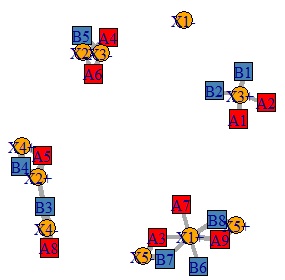
By the way, if the original data is directly converted into a bipartite graph, it will be as shown below. With this, it is difficult to think that there are "common elements".
NEXT  Many-to-many-to-many analysis (ABC type analysis)
