LiNGAM is a method that is explained as "it can be done with a non-normal distribution". So, this page is the one that I checked it.
First, the conclusion.
For the author, it is a surprising conclusion. It's a nice conclusion when I think about using it in practice.
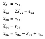
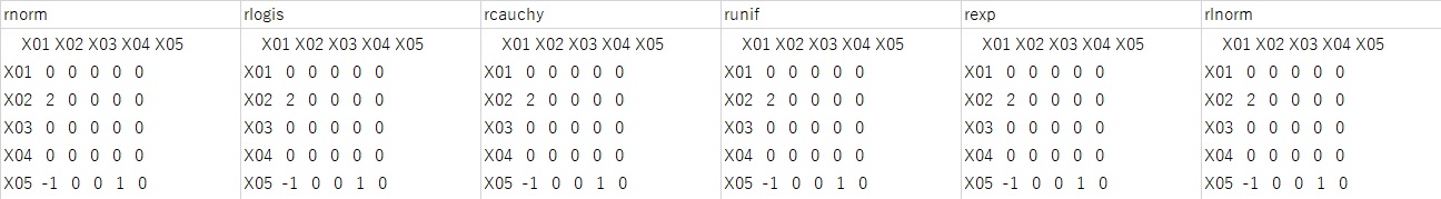
The formula of the model to be verified is as follows. If "2", "1", and "-1" appear once in the LiNGAM output matrix, and all others are "0", the answer is correct.
A random number with the specified distribution is entered in place of e. Each of the five e's is independent.
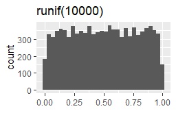
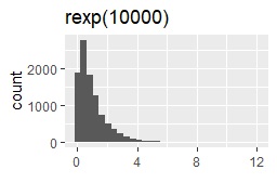
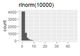
The distributions I tried this time are normal distribution, logistic distribution, Cauchy distribution, uniform distribution, exponential distribution and lognormal distribution. Create each with the codes rnorm (10000), rlogis (10000), rcauchy (10000), runif (10000), rexp (10000), rlnorm (10000). As you can see from this notation, the parameters for each distribution are left at their defaults. (The distribution is selected so that no error occurs even if no parameters are set.)
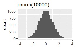
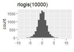
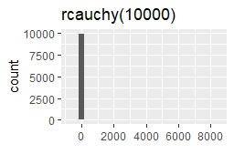
The code is below. Depending on the distribution, rewrite the "rnorm (10000)" part below.
e01 <- rnorm(10000)
e02 <- rnorm(10000)
e03 <- rnorm(10000)
e04 <- rnorm(10000)
e05 <- rnorm(10000)
X01 <- e01
X02 <- 2 * X01 + e02
X03 <- e03
X04 <- e04
X05 <- X04 - X01 + e05
Data <- as.data.frame(cbind(X01,X02,X03,X04,X05))
The code is below. " It's almost the same as the LiNGAM by R.
Below is the code that uses pcalg.
library(pcalg)
Str <- lingam(Data)$Bpruned
rownames(Str) <- colnames(Data)
colnames(Str) <- colnames(Data)
round(Str,1)
The code of my own work is also below for the pcalg part. The first two lines of the above code have been rewritten.
library(fastICA)
n <- ncol(Data)
fICA <- fastICA(Data, n)
K <- fICA$K
W <- fICA$W
tKW <- t(K %*% W)
MintKW <- tKW
MinSum <- sum(diag(1/abs(tKW)))
for (i in 1:10000) {
tKW2 <- tKW[order(sample(tKW,n)),]
SumdiagRabstKW <- sum(diag(1/abs(tKW2)))
if(MinSum > SumdiagRabstKW){
MinSum <- SumdiagRabstKW
MintKW <- tKW2
}
}
MintKW2 <- MintKW
for (i in 1:n) {
MintKW2[i,] <- MintKW2[i,]/MintKW2[i,i]
}
Str <- MintKW2
diag(Str) <- 0
rownames(Str) <- colnames(Data)
colnames(Str) <- colnames(Data)
round(Str,1)
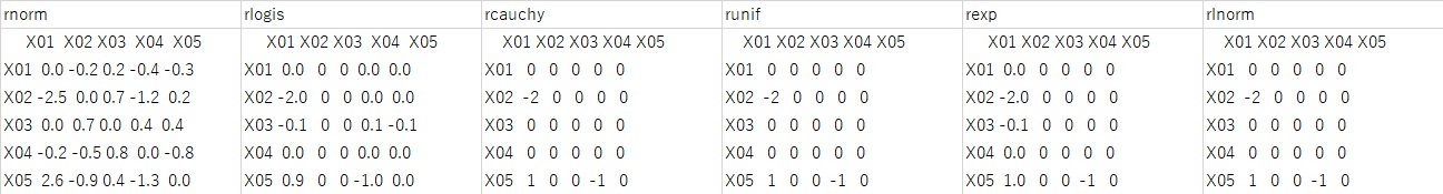
First, the result is something other than the normal distribution. All distributions are correct.
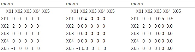
Next, the result for the normal distribution is shown in the figure below. The three results in the figure below are three examples of many trials.
Only the leftmost answer is correct, and the other two are incorrect in one of "2", "1", and "-1".
When I tried it, in the case of the normal distribution, the answer was wrong at a rate of about 1 out of 20 to 30 times.
This happens even with the exact same dataset, just by repeating the "lingam" code, so it's probably due to the randomness part of the ICA calculation in the lingam.
In conclusion , LiNGAM can be a useful method even when the distribution is normal, if you try it about 10 times and adopt the result that is reproduced many times regardless of whether the distribution is known or not .
At the time of normal distribution, it didn't work at all. In the case of other distributions, although there is an error of about 0.1, all the results are correct.
In the above experiment, the number of samples is 10,000. If you set this to 100 and execute the case of pcalg, the result shown in the figure below will be obtained.
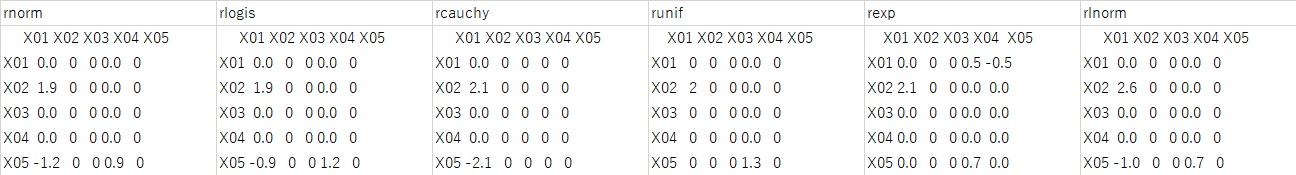
It is not a random number, and although the result is close to the correct answer to some extent, there are times when it is 0 where you do not want it to be 0.
When the number of samples is about several hundred, it seems good to consider the possibility that the correct answer is 0 instead of 0 as a risk.
NEXT  Principal Component Analysis
