factory_sensor01 is the data when manufacturing at the factory. As far as I know, this data is usually the secret of the factory. The data on this page was created by the author so that it has a shape close to a typical pattern.
This page is an example of analysis with R-EDA1 from the perspectives of "what is this data?" And "what can be learned from this data?" .
Since R-EDA1 is not all-purpose, we plan to use EXCEL together.
You can download the csv file saved in this site at the link of factory_sensor01.csv . The saved file is "factory_sensor01.csv", but it may be downloaded as a file called "factory_sensor01.xls" and an error message may appear that means "the extension is incorrect". In that case, change the extension of the downloaded file from "xls" to "csv" and you can use it without any problem.
From here, I'm using a file called "factory_sensor01.csv" in any location.
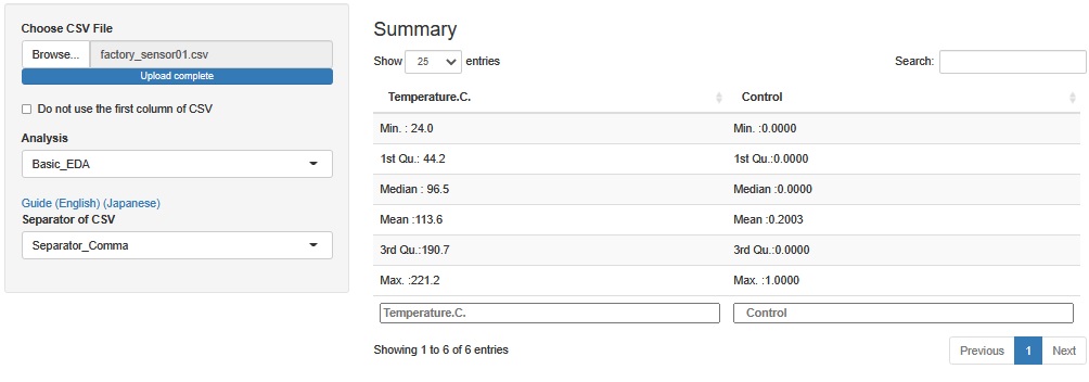
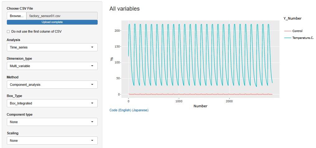
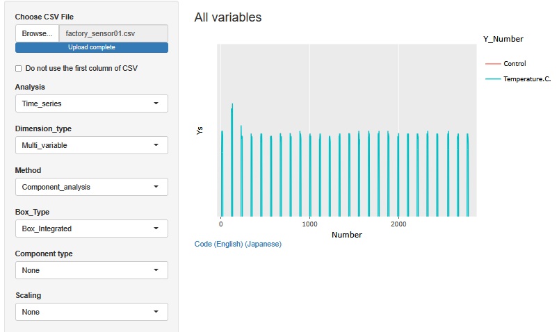
There are two variables, Temperature.C. and Control. Temperature.C. has a maximum of 221.2[C] and a minimum of 24.0[C] Control contains two values, 1 and 0.
The maximum temperature is about the same as the temperature at which bread and baked goods are baked. The lowest temperature is about the temperature.
The mountain of Temperature.C. is repeating. This one mountain represents one process. It is called a batch process, and this one process is the processing of one or a set of products.
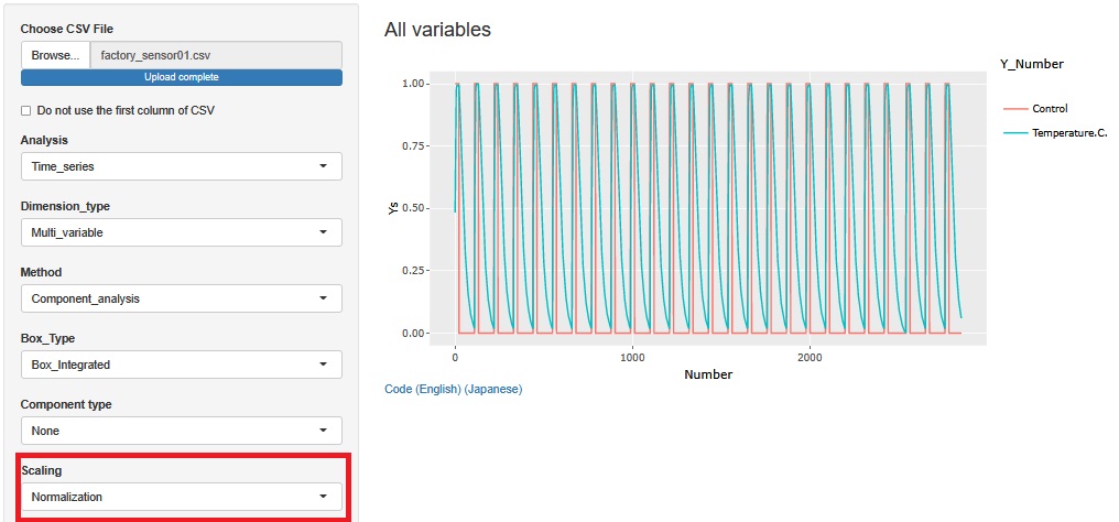
Normalization makes it easier to see what the Control variables look like.
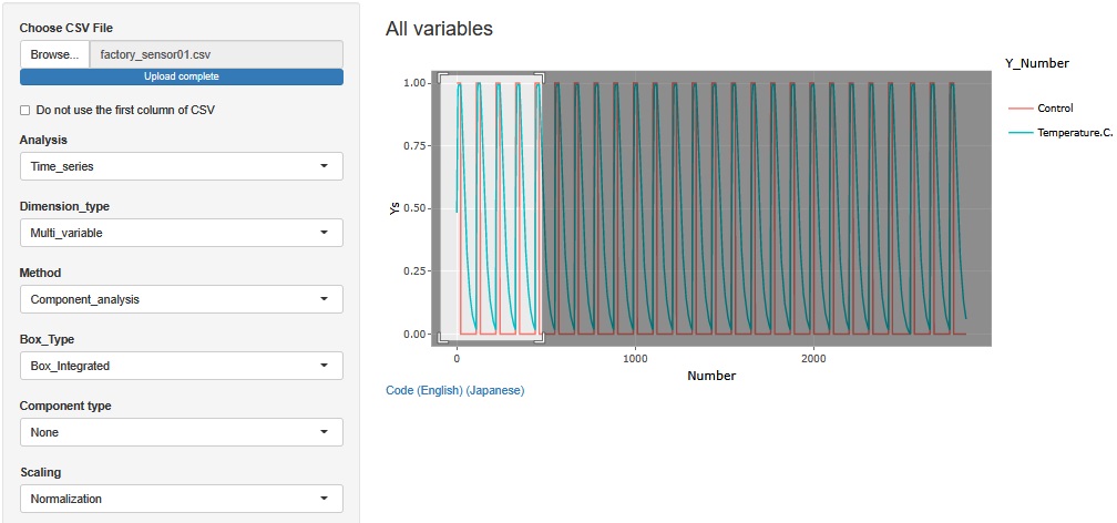
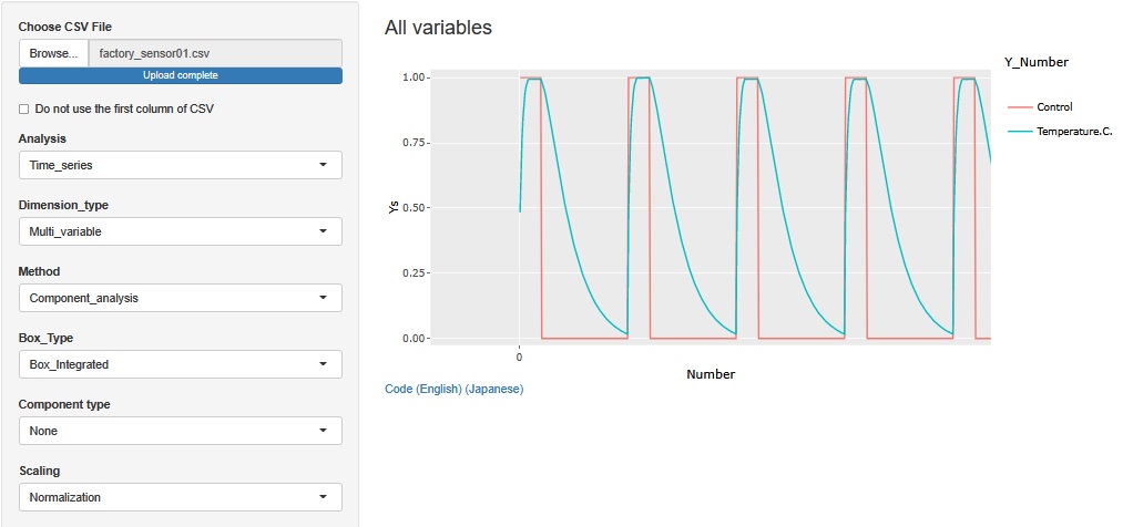
If you zoom in partially, you can see the relationship between the two variables. While Control was 1, Temperature.C. continued to rise, maintained at its maximum for a while, and then began to fall when it changed to 0.
I can see from the above that the waveform is repeating, but it seems unlikely that it will be any more. Therefore, Analysis of Type 2 (Feature Data) are created by repeatedly totaling the data once.
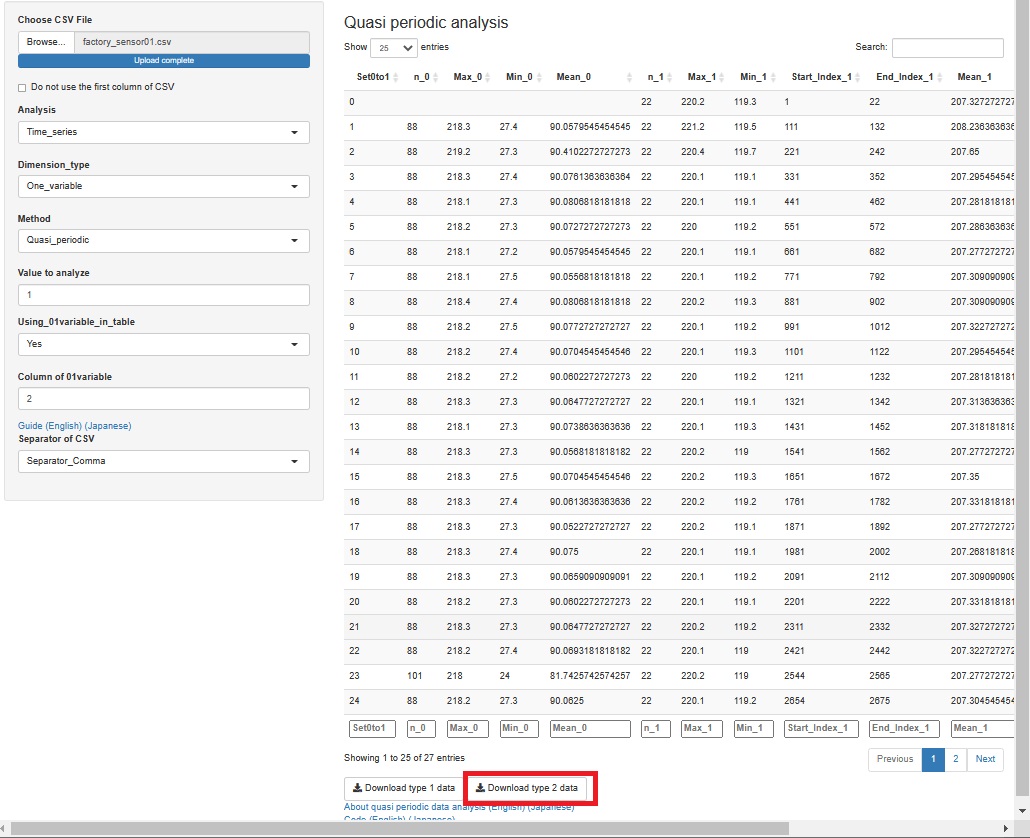
Regarding the settings in the figure below, first, since the variable to be analyzed is in the first column of Temperature.C., "Temperature.C." is set to "1". Also, I want to take advantage of the fact that the Control in the second column is repeated with 0 and 1, so I set "Using_01variable_in_table" to "Yes" and "Column of 01variable" to "2".
If you can set it, the total result will be displayed. You can analyze this result by looking at it, but if you want to see it in the graph, press "Dwonload type 2 data" at the bottom.
In many data analyses, the time between "1" is important for making the quality of manufacturing, so it is rare to find out by looking at the time of "0". However, what happened at "0" may have an effect at "1", or an invisible change at high temperature may be visible at low temperature, so make it a feature even at "0". It is good to leave it.
As a way to organize batches, there is also a method of summarizing in one line as one batch with "11111 ... 100000 ... 0", but if you do so, the change at the time of "0" has an effect. In order to avoid noticing this, R-EDA1 uses "00000 ... 011111 ... 1" and aggregates them into one line as one batch.
The original data starts at "1", so the first batch will never have a "0". Therefore, n_0, Max_0, Min_0, and Mean_0 in the first batch are missing values.
Depending on the device you are using, in my case, the downloaded file is saved in a folder called "Download".
With the horizontal axis in the first column, make a scatter plot of the relationship with all variables in the second and subsequent columns. Since the first column is the order of batches, it is a time series analysis of aggregated data for each batch.
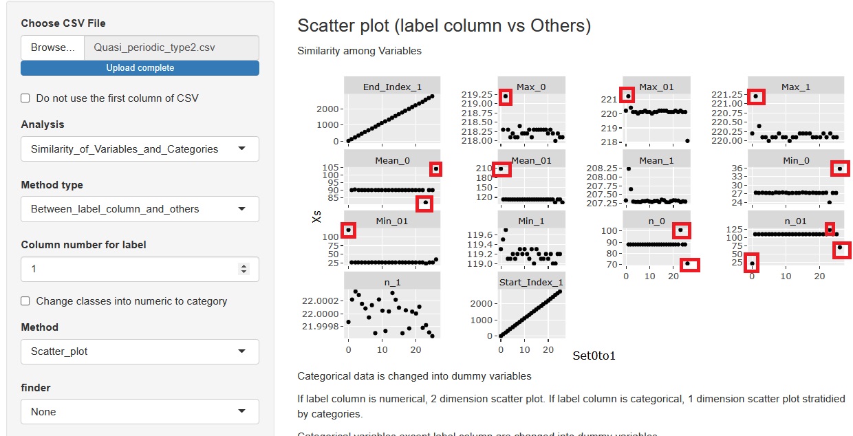
You can see that there are outliers here and there. In the analysis after this, for example, if phenomena such as "defective product is generated" and "foreign matter is generated" occur in one batch, we will investigate where the timing of that batch will be. If the timing of the batch matches the timing of outliers somewhere, it is possible that there is some relationship between the phenomenon and the outliers. Then that was a hint, what happened to the machine? What did you do to the machine? , And so on.
In addition, the first and last batches may lack data for one batch, and outliers are likely to occur. Therefore, it is a good idea to prepare the data so that the timing of the abnormality does not become the first or last batch.
Since the maximum temperature is different in the secondary data, let's graph the first data again. And expand the upper part.
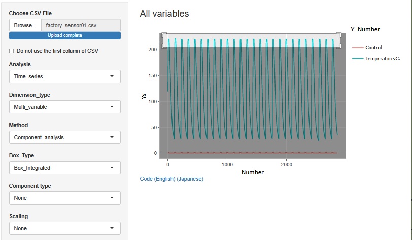
Then, you can see that the maximum temperature of the second batch is higher than that of the other batches.
When you create secondary data, you can easily notice that it is difficult to notice with the original data. Then, reviewing the original data will give you a better understanding of what is happening.
In factory_sensor01, in addition to the Temperature variable, there is a variable called Control, which is 0 and 1, and you can see the repetition of the batch, so it is used for batch aggregation.
Depending on the machine, variables like Control may be recorded as variables that literally represent the state of Control.
If there is no such variable and only Temperature, use the method of repeating Temperature.
First, set "Using_01variable_in_table" to "No". Also, set "Column to divide 0 or 1" to "1" in the Temperature.C. column. Then, in "Value to divide 0 or 1", enter a number to divide by temperature. For example, if you set it to "50", it will be as shown in the figure below. When set to "50", a new variable is created in which a variable higher than 50 becomes "1" and a variable lower than 50 becomes "0".
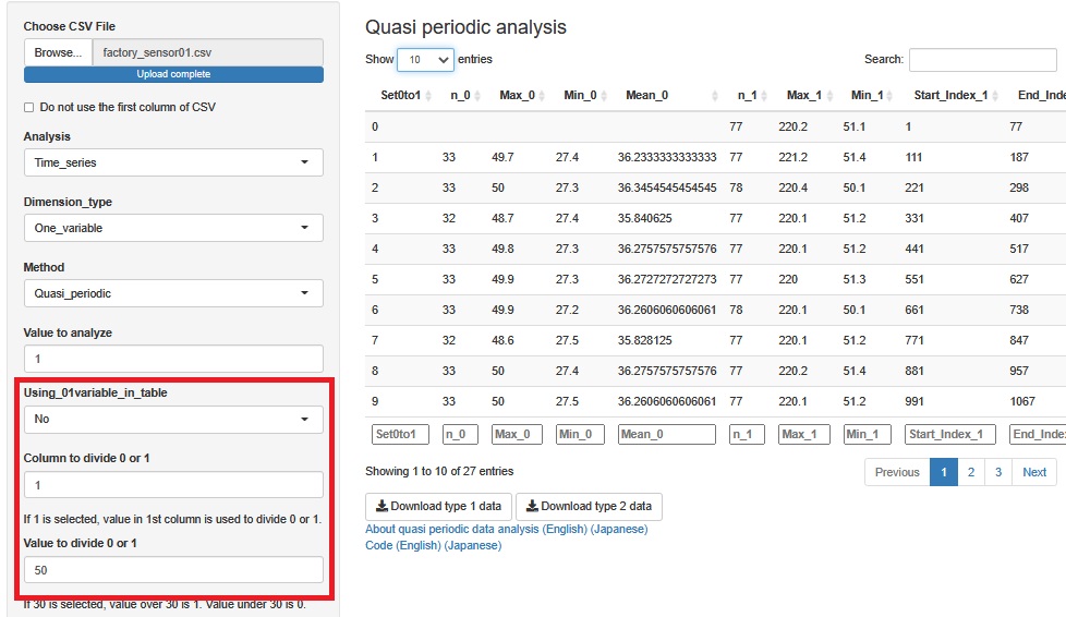
This function can be used not only when there is no 0-1 variable, but also as a way to cut out the section you want to pay attention to.
The quadratic data (features) that can be created with R-EDA1 can be easily created with built-in functions. There are many situations where this alone is useful.
However, when it comes to a more complicated phenomenon, it is no longer possible to say "easily with R-EDA1", and it is necessary to program using R, Python, VBA, etc. to create effective secondary data.
Actual factory data has more complex waveforms, and the shape of the waveform can have manufacturing implications. There may be several steps in the temperature, and it may be important to lower the temperature.
If there is a variable related to temperature, for example, the feature "value of that variable at the timing when it changes from 0 to 1" may be useful.
factory_sensor01 is about 3000 rows of data. Even with this, it may take several seconds to create the secondary data. (I think improving the processing speed is an issue for the future.)
Actual sensor data usually has more digits than this, but it is better not to try all of them suddenly.
It is more efficient and reliable to analyze by narrowing down the analysis period, such as "when a problem is occurring and when it is not occurring".
As a knack for processing large data, it is better to read the csv file at the end after reading the csv file, not in the order of specifying the variable numbers etc. Otherwise, R-EDA1 will start recalculation every time the value of the setting changes, so the already time-consuming process will be ordered one after another and it will freeze.
