library(survival)
Data <- read.csv("Data.csv", header=T)
ge.sf<-survfit(Surv(time,cens)~1, data=Data) plot(ge.sf,xlab="Time", ylab="Overall Survivial")
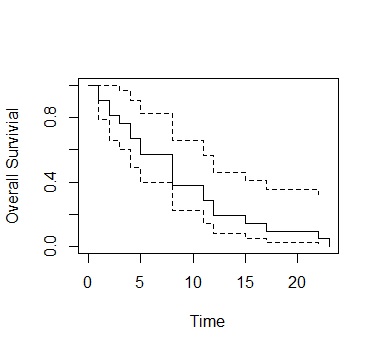
Dotted line is the confidence interval
This is an example of Survival Analysis by R.
The following is written as a memo of the code and is not as detailed as "analysis".
The data used in the code below is a csv file of R sample data called "gehan" and placed on the local PC.
The variable names are as follows.
time : survival time
cens : 1 = complete data, 0 = censored data
treat : factor category data
setwd("C:/Rtest")
library(survival)
Data <- read.csv("Data.csv", header=T)
ge.sf<-survfit(Surv(time,cens)~1, data=Data)
plot(ge.sf,xlab="Time", ylab="Overall Survivial")
Dotted line is the
confidence interval
setwd("C:/Rtest")
library(survival)
Data <- read.csv("Data.csv", header=T)
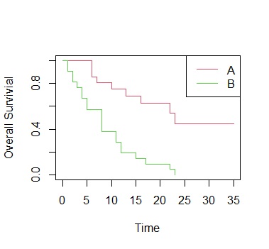
ge.sf<-survfit(Surv(time,cens)~treat, data=Data)
plot(ge.sf, col=2:3,xlab="Time", ylab="Overall Survivial")
legend("topright", paste(c("A","B")), lty=1, col=2:3)
setwd("C:/Rtest")
library(survival)
Data <- read.csv("Data.csv", header=T)
summary(survreg(Surv(time,cens)~1,Data,dist="weibull"))
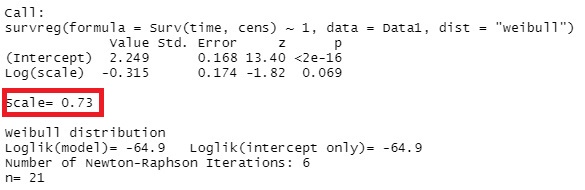
As for how to read this result, the shape parameter often explained by the symbols "m" and "Beta" is the reciprocal of the numerical value "Scale". In this example, it is 0.73, but the reciprocal is 1.37 (= 1 / 0.73), which is larger than 1, so it can be interpreted as the wear failure period (the period on the right side of the bathtub curve where the failure rate increases steadily). ..
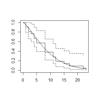
Create a graph that overlays the results calculated by the Kaplan-Meier method and the results calculated by the Weibull analysis.
In R, it's easy to make a Kaplan-Meier graph. Weibull analysis, on the other hand, has more complex code. After a lot of research, the content of the references below was the simplest. This method makes it easy by creating a graph of the Kaplan-Meier method and then overlaying it.
setwd("C:/Rtest")
library(survival)
Data <- read.csv("Data.csv", header=T)
sr <- survreg(Surv(time,cens)~1,Data,dist="weibull")
sf <-survfit(Surv(time,cens)~1, Data)
plot(sf)
curve(1-pweibull(x,shape=1/sr$scale, scale=exp(coef(sr)[1])),add=TRUE)
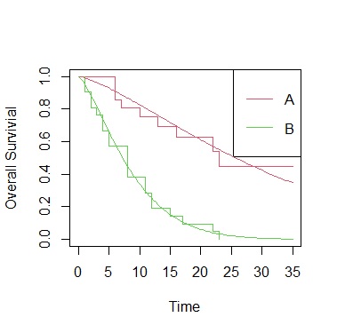
setwd("C:/Rtest")
library(survival)
Data <- read.csv("Data.csv", header=T)
sr <- survreg(Surv(time,cens)~treat,Data,dist="weibull")
sf <- survfit(Surv(time,cens)~treat, Data)
plot(sf, col=2:3,xlab="Time", ylab="Overall Survivial")
legend("topright", paste(c("A","B")), lty=1, col=2:3)
curve(1-pweibull(x,shape=1/sr$scale, scale=exp(coef(sr)[1])),add=TRUE, col=2)
curve(1-pweibull(x,shape=1/sr$scale, scale=exp(coef(sr)[1]+coef(sr)[2])),add=TRUE, col=3)
setwd("C:/Rtest")
library(survival)
Data <- read.csv("Data.csv", header=T)
summary(coxph(Surv(time, cens) ~ treat, data=Data))
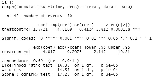
In the above example, there is only one factor variable, treat. For example, if you have a variable called treat2 and want to add it to the factor, write treat + treat2.
