Data Analysis by R

Correspondence analysis by R

This is an example of Correspondence analysis by R.

Correspondence analysis starting from the data in the contingency table

It is in Analysis of similarity between items in rows and columns by R.

Multiple correspondence analysis

This is an example of Multiple correspondence analysis.

Creating data for graphs

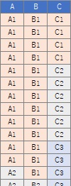
In this example, it is assumed that the folder "Rtest" on the C drive contains the data that is a contingency table with the name "Data.csv".

library(dummies)
library(MASS)
setwd("C:/Rtest")
Data <- read.csv("Data.csv", header=T)
Data_dmy <- dummy.data.frame(Data)
pc <- corresp(Data_dmy,nf=min(ncol(Data_dmy)))
pc1 <- pc$cscore
pc1 <- transform(pc1 ,name1 = rownames(pc1))
round(pc$cor^2/sum(pc$cor^2),2)# Calculate the contribution rate.
�@

In the above example, the 7th and subsequent eigenvalues ??have a low contribution rate, so we will exclude them from the subsequent analysis.

Multidimensional scatter plot

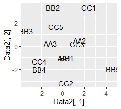
A multidimensional scatter plot is a scatter plot that allows you to see multiple dimensions in two dimensions. It is equivalent to the AB type multidimensional simultaneous attachment diagram . Starting with qualitative data eliminates the need for a procedure to combine both row-side and column-side calculation results.

MaxN = 6# Specify the number of unique values to use
Data11 <- pc1[,1:MaxN]
Data11_dist <- dist(Data11)
sn <- sammon(Data11_dist)
output <- sn$points
Data2 <- cbind(output, pc1)�@
library(ggplot2)
ggplot(Data2, aes(x=Data2[,1], y=Data2[,2],label=name1)) + geom_text()

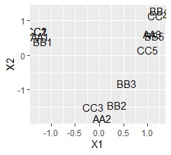
By the way, if you make a graph with the first and second components of correspondence analysis, it will be as follows, and it is not possible to separate.

Applued Bipartite graph

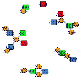
There is one more place to set the color, but the method of making is basically the same to the bipartite graphs.

MaxN = 6
library(igraph)# specifies the number of eigenvalues to use
library(sigmoid)
Data1p = pc1[,1:MaxN]
names(Data1p) = paste(names(Data1p),"+",sep="")
DM.matp = apply(Data1p,c(1,2),relu)
Data1m = -pc1[,1:MaxN]
names(Data1m) = paste(names(Data1m),"-",sep="")
DM.matm = apply(Data1m,c(1,2),relu)
DM.mat =cbind(DM.matp,DM.matm)
DM.mat <- DM.mat / max(DM.mat) * 10
DM.mat[DM.mat < 3] <- 0
DM.g<-graph_from_incidence_matrix(DM.mat,weighted=T)
V(DM.g)$color <- c("steel blue", "orange")[V(DM.g)$type+1]
V(DM.g)$color[1:3] <- "red"
V(DM.g)$color[4:8] <- "green"
V(DM.g)$shape <- c("square", "circle")[V(DM.g)$type+1]
plot(DM.g, edge.width=E(DM.g)$weight)

Tweet