The theory of estimation may be something that people who use statistics on a regular basis do not use at all. In my case, the theory of confidence intervals has never been useful, but the prediction intervals have been useful several times.
This is an application of Software for Prediction .
This example is how to find the 95% prediction interval.
The example of the prediction interval on the estimation page is to be executed in R.
An example of using R is as follows. The following is copy paste and can be used as it is. In this example, it is assumed that there is a file called "Data.csv" in the folder called "Rtest" on the C drive, and the data is stored only in the first column. It is assumed that the numerical data is included from the first line and the variable name is not included.
The plus and minus signs on the upper and lower sides of the prediction interval seem to be the opposite of the formula on the estimation page, but this is done according to the specifications of the function qt.
setwd("C:/Rtest")
Data <- read.csv("Data.csv", header=F)
M <- mean(Data[,1])
n <- nrow(Data)
t <- -qt((1-0.95)/2, n-1)
V <- var(Data[,1])
Upper <- M + t * sqrt(V * (1 + 1/n)) # Upper of interval
Lower <- M - t * sqrt(V * (1 + 1/n)) # Lower of interval
Upper# Output of Upper
You can also estimate the Prediction Interval of Regression Analysis .
An example of using R is as follows. The following is copy paste and can be used as it is. In this example, it is assumed that the folder named "Rtest" on the C drive contains data with the name "Data.csv".
It is also assumed that the data contains a variable named "Y" as the objective variable and "X" as the explanatory variable.
setwd("C:/Rtest")
Data <- read.csv("Data.csv", header=T)
lm <- lm(Y ~ ., data=Data)
X <- 6 # Enter
the value of X for which you want to find the prediction interval
X <- as.data.frame(X)
predict(lm, X , interval="prediction", level = 0.95)
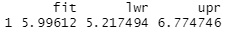
The predicted value obtained in the regression equation (fit), the upper prediction interval (upr), lower (LWR) is output.
For example, "Since the upper side is 6.77, when X = 6, if Y = 6, it is a normal value. If Y = 7, it is an abnormal value ."
library(ggplot2)
setwd("C:/Rtest")
Data <- read.csv("Data.csv", header=T)
lm <- lm(Y ~ ., data=Data)
Data1 <- predict(lm, Data, interval="prediction", level = 0.95)
Data2 <- cbind(Data, Data1)
ggplot(data = Data2, aes(x = X, y = Y)) +geom_point()+geom_line(aes(y=lwr), color = "red")+geom_line(aes(y=upr), color = "red")+geom_line(aes(y= fit), color = "blue")
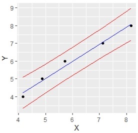
In this graph as well, for example, "when X = 6, if Y = 6, the normal value. If Y = 7, the abnormal value ", the point that can be used to judge the abnormal value is the same.
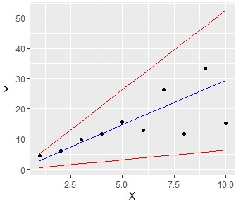
The case for Prediction interval of Proportional variance .
library(ggplot2)
setwd("C:/Rtest")
Data <- read.csv("Data.csv", header=T)
M <- mean(Data$Y / Data$X)
n <- nrow(Data)
t <- -qt((1-0.95)/2, n-1)
V <- var(Data$Y / Data$X)
Upper <- M + t * sqrt(V * (1 + 1/n))
Lower <- M - t * sqrt(V * (1 + 1/n))
upr<-Data$X * Upper
lwr<-Data$X * Lower
fit<-Data$X * M
Data2<-cbind(Data,lwr,upr,fit)
ggplot(data = Data2, aes(x = X, y = Y)) +geom_point()+geom_line(aes(y=lwr), color = "red")+geom_line(aes(y=upr), color = "red")+geom_line(aes(y= fit), color = "blue")