Visualization by compressing high-dimensional into two dimensions with regression analysis system by R
Visualization by compressing high dimensions into two dimensions with regression analysis and Residual Outliers An example according to R.
Example of execution
In the example data, the first column variable is the objective variable Y. Data other than the first row is created by adding an error to the sum of the explanatory variables. Only the data in the first row, Y does not use this calculation and enters an appropriate value.
In the following, four regression analysis systems can be used. It might be interesting to be able to do it with AutoML. Note that "automl" in the code below is a package that automatically adjusts the parameters of the neural network. If you use automl, it will be automatic for neural networks, but it is not a way to try various other methods.
Compressed to 2D data
setwd("C:/Rtest")
library(ggplot2)
library(plotly)
Data <- read.csv("Data.csv", header=T)
Data1 <- Data
label_column <- 1
Y2 <- names(Data1[label_column])
Y2data <- Data1[,label_column]
Data1[Y2] <- NULL
Data4<-cbind(Y2data,Data1)
#Making model
Dimension_Reduction_Method2 <- 1 # 1=regression analysis, 2=model tree, 3=SVR, 4=neural network
if(Dimension_Reduction_Method2 == 1) {
two_demension_model <- step(glm(Y2data~., data=Data4, family= gaussian(link = "identity")))
} else if(Dimension_Reduction_Method2 == 2) {
library(Cubist)
two_demension_model <- cubist(y = Y2data, x=Data1, data = Data4, control=cubistControl(rules = 5))
} else if(Dimension_Reduction_Method2 == 3) {
library(kernlab)
two_demension_model<- ksvm(Y2data~.,data=Data4,type='eps-svr', kernel="rbfdot")
} else if(Dimension_Reduction_Method2 == 4) {
library(automl)
two_demension_model<- automl_train(Data1,Y2data)
}
#Estimation
if(Dimension_Reduction_Method2 == 4) {
s2 <- automl_predict(two_demension_model,Data1)
} else {
s2 <- predict(two_demension_model,Data1)
}
Data6 <- cbind(data.frame(Y2data,s2),Index = row.names(Data))
#graph
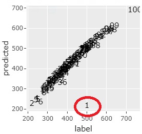
ggplotly(ggplot(Data6, aes(x=Data6[,1], y=Data6[,2],label=Index)) + geom_text() + labs(y="predicted",x="label"))
Analyzing Residuals
The analysis of outliers in the residuals adds: There are two examples of graphing.
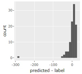
Y1 <- s2 - Y2data# residuals
ggplotly(ggplot(Data, aes(x=Y1)) + geom_histogram()+ labs(x="predicted - label"))# histgram
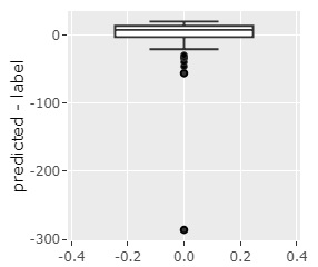
ggplotly(ggplot(Data, aes(y=Y1)) + geom_boxplot() + labs(y="predicted - label"))# box plot
Checking the Model
Regression analysis and model trees provide simple models. You can see what kind of model it has become below.
summary(two_demension_model)
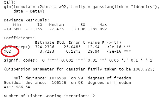
In this example, you can see that the model was created with only an explanatory variable called X02.
