Canonical Correlation Analysis by R
Example of
Canonical Correlation Analysis
and
Visualization by compressing high dimensions into two dimensions with Canonical Correlation Analysis
.
Ordinary canonical correlation analysis
In the example data, there are 6 variables, and it is assumed that the 3 from the left and the 3 after that are each a group.
In the same way that principal component analysis computes multiple synthetic variables, the first principal component, the second principal component, and so on, multiple synthetic variables are computed in canonical correlation analysis. In the example below, only the combination of the first component is extracted and made into a scatter diagram.
CCA library
setwd("C:/Rtest")
library(CCA)
library(ggplot2)
library(plotly)
Data <- read.csv("Data.csv", header=T)
Retu <- 3 # Columns 1:3 is one group. Other columns is the other group
DataX <- Data[,1:Retu]
Retu2 <- Retu+1
Retu3 <- ncol(Data)
DataY <- Data[,Retu2:Retu3]
model <- cc(DataX,DataY)
Youso <- 1# Number of factor
X1 <- model$scores$xscores[,Youso]
Y1 <- model$scores$yscores[,Youso]
Data5 <- cbind(data.frame(X1,Y1),Index = row.names(Data))
ggplotly(ggplot(Data5, aes(x=X1, y=Y1,label=Index)) + geom_text() + labs(x="Xs",y="Ys"))
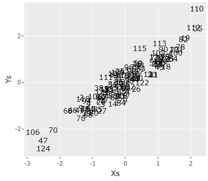
model$cor# Correlation coefficient

We can see that the first components have a correlation coefficient of 0.93. The second component is also high because it is 0.87.
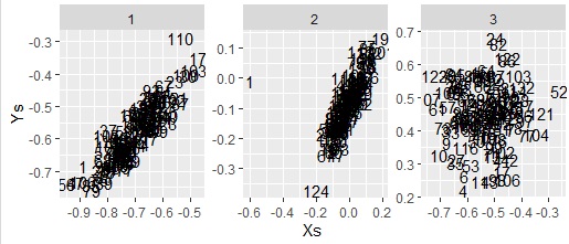
cancor function
The cancor function is standard installed with R. Basically the same as CCA, but new components are not calculated and must be calculated from the coefficients.
setwd("C:/Rtest")
library(ggplot2)
library(plotly)
Data <- read.csv("Data.csv", header=T)
Retu <- 3 # Columns 1:3 is one group. Other columns is the other group
DataX <- Data[,1:Retu]
Retu2 <- Retu+1
Retu3 <- ncol(Data)
DataY <- Data[,Retu2:Retu3]
model <- cancor(DataX,DataY)
u <- data.matrix(DataX) %*% model$xcoef
v <- data.matrix(DataY) %*% model$ycoef
Data6 <- cbind(u = data.frame(u[,1]),v = data.frame(v[,1]),Index = row.names(Data),Factors = c(1))
names(Data6)[1:2] <- c("u","v")
for(i in 2:min(ncol(u),ncol(v))) {
Data61 <- cbind(u = data.frame(u[,i]),v = data.frame(v[,i]),Index = row.names(Data),Factors = c(i))
names(Data61)[1:2] <- c("u","v")
Data6 <- rbind(Data6,Data61)
}
ggplot(Data6, aes(x=u,y=v,label=Index)) + geom_text() + facet_wrap(~Factors,scales="free") + labs(x="Xs",y="Ys")
Kernel canonical correlation analysis (nonlinear)
In the example data, there are 6 variables, and it is assumed that the 3 from the left and the 3 after that are each a group.
kernlab library
setwd("C:/Rtest")
library(kernlab)
library(ggplot2)
library(plotly)
Data <- read.csv("Data.csv", header=T)
Retu <- 3 # Columns 1:3 is one group. Other columns is the other group
DataX <- Data[,1:Retu]
Retu2 <- Retu+1
Retu3 <- ncol(Data)
DataY <- Data[,Retu2:Retu3]
k <- rbfdot()# laplacedot(), besseldot(), anovadot(), splinedot(), polydot(), vanilladot(), tanhdot()
result <- kcca(data.matrix(DataX), data.matrix(DataY), kernel = k, ncomps = 3)
u <- kernelMatrix(k,data.matrix(DataY)) %*% result@xcoef
v <- kernelMatrix(k,data.matrix(DataX)) %*% result@ycoef
Youso <- 1# Number of factor
Y1 <- u[,Youso]
X1 <- v[,Youso]
Data5 <- cbind(data.frame(X1,Y1),Index = row.names(Data))
ggplotly(ggplot(Data5, aes(x=X1, y=Y1,label=Index)) + geom_text() + labs(x="Xs",y="Ys"))
