This is an example of Item Response Theory by R.
How to find the coefficients of a model formula.
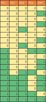
Here, the following data is used. It is assumed that the csv file of this data is in a folder called Rtest on the C drive.
setwd("C:/Rtest")
library(ltm)
Data <- read.csv("Data.csv", header=T)
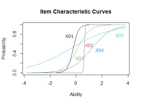
ltmModel <- ltm(Data ~ z1)
plot(ltmModel)
ltmModel <- ltm(Data ~ z1+z2)
is set here,
two latent variables will be created. In this library, 3 or more (z3 etc.) cannot be set.
ltmModel <- ltm(Data ~ z1*z2)
is set here,
the interaction term between z1 and z2 will also appear.
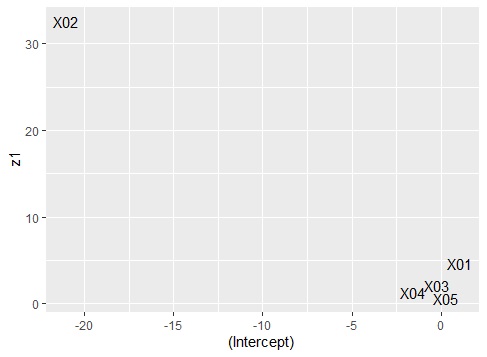
The graph above gets messed up when there are a lot of variables. It is easier to consider each variable if you make a scatter plot with the two coefficients of the logistic function. You can see the meaning of the coefficients by comparing the curve and the scatter plot.
Data2 <- as.data.frame(ltmModel$coefficients)
library(ggplot2)
ggplot(Data2, aes(x=Data2[,1], y=Data2[,2],label=row.names(Data2))) + geom_text() +xlab("(Intercept) ")+ylab("z1")
How to find out the score of a sample.
Data3<-factor.scores(ltmModel)
Dat3$score.dat
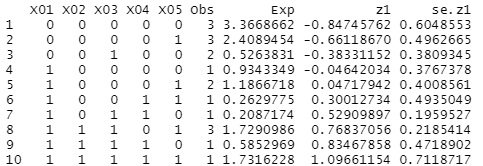
The score of the sample is a variable called "z1". You can see that the more correct answers (1), the higher the score.
The variable "obs" represents the number of samples of the same data. With this library, it is inconvenient to think "What is the fifth score of the original data?" Because it is summarized by a sample of the same data. I tried to find a solution, but I don't know so far.
setwd("C:/Rtest")
library(ltm)
Data <- read.csv("Data.csv", header=T)
ltmModel <- grm(Data)
plot(ltmModel)
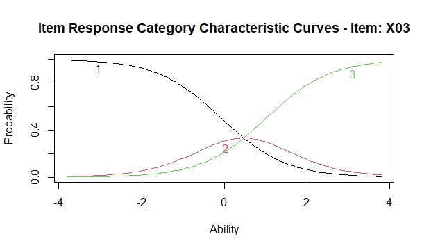
In GRM, plots are made for each variable.
Process after is same to the bainary data model.
CRAN
https://cran.r-project.org/web/packages/ltm/ltm.pdf
Manual of ltm
