Multi Dimensional Scaling is a technique that everyone in the know knows, but it is convenient. It can be used in important parts even though it is inconspicuous.
There are several multidimensional scaling methods, and in the example of R below, the method is called sammon, but in the case of cmdscale, the results are the same as the Principal Component Analysis . If you want to group samples on a 2D map, I think the multidimensional scaling method with sammon is good.
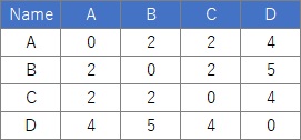
This is an example of multidimensional scaling using R. The following is copy paste and can be used as it is. This example assumes that the input data is quantitative data. An error will occur if there is qualitative data.
In this example, it is assumed that the folder named "Rtest" on the C drive contains data with the name "Data1.csv".
library(MASS)
library(som)
library(ggplot2)
setwd("C:/Rtest")
Data1 <- read.csv("Data1.csv", header=T)
Data11 <- Data1[,2:5]# Specify a column with distance data. This example is for columns 2-5
Data11_dist <- as.matrix(Data11)
sn <- sammon(Data11_dist)
output <- sn$points
Data <- cbind(output, Data1)
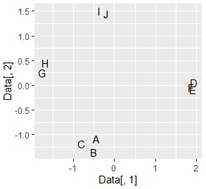
ggplot(Data, aes(x=Data[,1], y=Data[,2],label=Name)) + geom_text()
A, B, C groups and D It should be divided into independent parts, and it's almost like that.
In this example, it is assumed that the folder named "Rtest" on the C drive contains data with the name "Data1.csv".
library(MASS)
library(som)
setwd("C:/Rtest")
Data1 <- read.csv("Data1.csv", header=T)
Data11 <- normalize(Data1[,1:3],byrow=F)
Data11_dist <- dist(Data11)# Calculate the distance between samples
sn <- sammon(Data11_dist)
output <- sn$points
Data <- cbind(output, Data1)
Data$Index <-row.names(Data)
library(ggplot2)
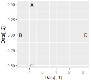
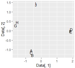
ggplot(Data, aes(x=Data[,1], y=Data[,2],label=Name)) + geom_text()
Divided into 4 groups as expected .
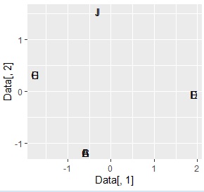
The figure on the left shows "cmdscale" instead of "sammon", and the figure on the right shows "isoMDS". It was the same that it was divided into 4 groups as expected, but in the case of isoMDS, the first 3 digits of the same group were placed so close that they became the same number. Therefore, the characters overlap in the graph.
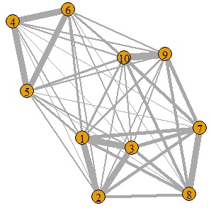
This is an example of Networked multidimensional scaling .
In this example, it is assumed that the folder named "Rtest" on the C drive contains data with the name "Data1.csv".
library(igraph)
setwd("C:/Rtest")
Data1 <- read.csv("Data1.csv", header=T)
Data11 <- Data1[,2:5]
Data12 <- as.matrix(Data11)
Data12 <- (max(Data12) - Data12)
diag(Data12) <- 0
Data12 <- Data12 / max(Data12) * 10
GM4 <- graph.adjacency(Data12,weighted=T, mode = "undirected")
plot(GM4, edge.width=E(GM4)$weight)
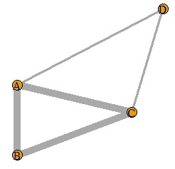
A, B, C It should be divided into the group of D and D alone, and it was almost like that.
When starting multidimensional data, it can be used as a Visualize by compressing high dimensions into two dimensions.
In this example, it is assumed that the folder named "Rtest" on the C drive contains data with the name "Data1.csv".
library(igraph)
setwd("C:/Rtest")
Data1 <- read.csv("Data1.csv", header=T)
Data10 <- Data1[,1:3]
Data11 <- (Data10 - apply(Data10,2,min))/(apply(Data10,2,max)-apply(Data10,2,min))# For all variables Make the data between 0 and 1.
Data12 <- as.matrix(dist(Data11))
Data12 <- (max(Data12) - Data12)
diag(Data12) <- 0
Data12 <- Data12 / max(Data12) * 10
hist(Data12)
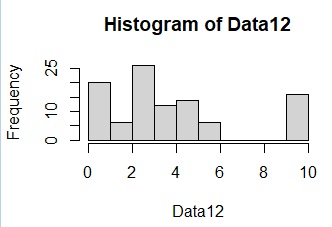
Data12[Data12< 8] <- 0
GM4 <- graph.adjacency(Data12,weighted=T, mode = "undirected")
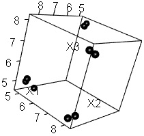
plot(GM4, edge.width=E(GM4)$weight)
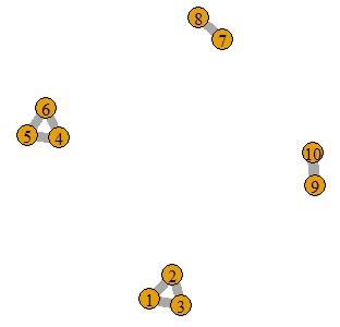
4 as expected Divided into groups.
The code for starting multidimensional data contains the code "0 if less than 8" by checking the data in the histogram. If you do not enter the code "0 if it is less than 8", it will be as shown in the figure below and it will be messed up. Originally, when using this method, it is time to find something close to it, so I think it's okay to cut the line with something far away. Even if you start the distance data, you can cut the line with the distant one in the same way.