Data Analysis by R

Analysis of the presence or absence of difference by R

The test can quantitatively analyze the question, "Is there a difference?"

Test for the difference between two population means

The test for the difference in mean values is one of the most basic tests. There are two columns of data, and it is assumed that the first and second columns are compared.

Student's t-test

setwd("C:/Rtest") #
Data <- read.csv("Data.csv", header=T) #
t.test(x=Data$X1,y=Data$X2,var.equal=T,paired=F) #

Welch's t-test

setwd("C:/Rtest")#
Data <- read.csv("Data.csv", header=T)#
t.test(x=Data$X1,y=Data$X2,var.equal=F,paired=F) #

Test for the difference between two or more population means

Up to two-way ANOVA, you can also use Excel's data analysis function.

One-way ANOVA

The data assumes that the first column has a column name of "X" and the category, and the second column has a column name of "Y" and contains numerical values.

setwd("C:/Rtest") #
Data <- read.csv("Data.csv", header=T)#
summary(aov(Y~X,data=Data))#

Two-way ANOVA (no interaction term)

The data assumes that the first and second columns have column names "X1" and "X2" with level names, and the third column has column names "Y" with numerical values.

setwd("C:/Rtest") #
Data <- read.csv("Data.csv", header=T)#
summary(aov(Y~X1+X2,data=Data)) #

Two-way ANOVA (with interaction term)

When evaluating the interaction , the "+" is replaced with "*".

Repeated data is required to include the interaction term. Repeated data means that there are multiple times of data for each combination of levels of the two factors.

setwd("C:/Rtest")#
Data <- read.csv("Data.csv", header=T) #
summary(aov(Y~X1*X2,data=Data)) #

Visualization of differences in mean and variability

Graph that decomposes one quantitative variable into one qualitative variable

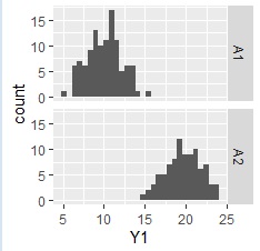
The data assumes that the column name "C1" contains the category and the column name "Y1" contains the number.

ggplot(Data, aes(x=Y1)) + geom_histogram() + facet_grid(C1~.)#

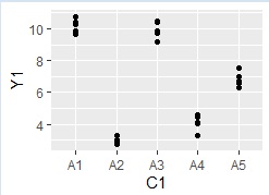
ggplot(Data, aes(x=C1, y=Y1)) + geom_point()#

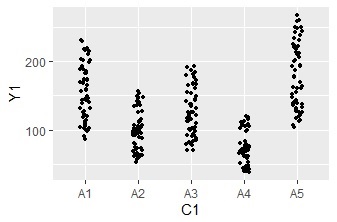
The size of the plot can be adjusted by size, and the degree of horizontal dispersion can be adjusted by the number of position = position_jitter.

ggplot(Data, aes(x=C1, y=Y1)) + geom_jitter(size=1, position=position_jitter(0.1))#

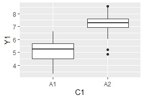
ggplot(Data, aes(x=C1, y=Y1)) + geom_boxplot()#

A graph that decomposes one quantitative variable into two qualitative variables

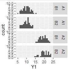
ggplot(Data, aes(x=Y1)) + geom_histogram() + facet_grid(C1+C2~.)#

ggplot(Data, aes(x=C1, y=Y1)) + geom_jitter(size=1, position=position_jitter(0.1)) +facet_grid(.~C2)#

Test of the difference between the paired means

Test for the difference between two paired means

setwd("C:/Rtest") #
Data <- read.csv("Data.csv", header=T) #
t.test(x=Data$X1,y=Data$X2,paired=T) #

est for the difference between three or more paired means

The data assumes that the first and second columns have column names "X1" and "X2", and the third column has column names "Y". "X2" is the character string that represents the correspondence.

setwd("C:/Rtest")#
Data <- read.csv("Data.csv", header=T)#
summary(aov(Y~X1+X2,data=Data))#

Test of population variance ratio (test of variation)

Test of the ratio of two population variances

The data assumes that there are two columns, the column names "X1" and "X2" are in the first row, and the numbers are below them. )

setwd("C:/Rtest")#
Data <- read.csv("Data.csv", header=T)#
var.test(x=Data$X1,y=Data$X2) #

Test for 3 or more (Bartlett's test)

The data assumes that the first column has a column name of "X" and the category, and the second column has a column name of "Y" and contains numerical values.

setwd("C:/Rtest")#
Data <- read.csv("Data.csv", header=T) #
bartlett.test(formula=Data$Y~Data$X) #

Test of ratio difference

In the case of the test of the difference between "1/10" and "4/20"

prop.test(c(1,4),c(10,20))#

Test of independence

It is a test of independence using the chi-square test .

setwd("C:/Rtest") #
Data <- read.csv("Data.csv", header=T)#
chisq.test(Data)#