An R implementation of variable importance analysis .
Although there is some overlap with the Generalized Linear Mixed Models in R page, this page focuses on the features of variable importance analysis. Variable selection features are useful in this analysis.
The example below is from a multiple regression analysis . Since it is a generalized linear model , logistic regression analysis can also be performed.
Generally, when it is said to be the "stepwise method", it is often the variable increase/decrease method.
library(MASS)
setwd("C:/Rtest")
Data1 <- read.csv("Data.csv", header=T)
gm <- step(glm(Y~., data=Data1, family= gaussian(link = "identity")),criteria = "AIC",direction = "both")
summary(gm)
For "direction = "both"", "both" (variable increase/decrease method), "backward" (variable decrease method,) and "forward" (variable increase method) can be selected. If you omit "direction="both"", it defaults to "both".
For "criteria = "AIC"", select "AIC", "AICc", "AICb1", "AICb2", "BIC", "KIC", "KICc", "KICb1", "KICb2" increase. If you omit "criteria = "AIC"", it defaults to "AIC".
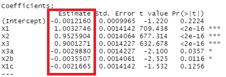
In the following example, we use data that is made like Y = X1 + 0.95 * X2 + 0.9 * X3 + E (error) . Other than X1, X2, and X3 are highly correlated with X1, X2, and X3, but are irrelevant to Y. The number of samples is 10,000.
The coefficients are calculated almost exactly.
X3a, X2b, and X1c are in, although I don't want them in there. Compared to X1, X2, and X3, the P-value is an order of magnitude larger, so in conclusion, it is possible to conclude that it is a formula determined by X1, X2, and X3, but it is judged to be "significant." In the stepwise method, the p-value is included in the judgment, so it is easy to get simple results when the number of samples is small. The larger the number of samples, the more likely it is to be significant, so it is less likely that you will say, "This variable is not included."
By default, the glmnet package includes a function to normalize the explanatory variables before executing. Therefore, the coefficients obtained are standard partial regression coefficients, which can be used to assess the influence of variables.
library(glmnet)
setwd("C:/Rtest")
Data1 <- read.csv("Data.csv", header=T)
Y <- Data1$Y
Data1$Y <- NULL
lasso.cv <- cv.glmnet(x = as.matrix(Data1), y = Y, family = "gaussian", alpha = 1)
lasso <- glmnet(x = as.matrix(Data1), y = Y, family = "gaussian", alpha = 1,lambda = lasso.cv$lambda.min) d
lasso$beta# Ś‹‰Ę‚ĚŹo—Í
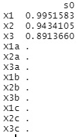
The output is the coefficients of the regression equation.
For "family = "gaussian"", you can choose "gaussian", "binomial", "poisson", "multinomial", "cox", "mgaussian". Similar to the glm function above. For "gaussian", it is a multiple regression analysis.
The da
ta are the same as for the stepwise method above.
Except for X1, X2, and X3, all are 0, and the three variables are extracted cleanly.
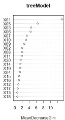
A decision tree is originally based on the idea of ??trying to express the objective variable with as few variables as possible.
Therefore, decision trees in R can be used for variable importance analysis.
Random forests can create many models with few variables, but the ability to aggregate them is also included in R's random forests.