Analysis of hidden variables by R
This is a recipe for exploring hidden variables with R.
I wanted to search for a hypothesis by correlation as a causal inference , and I analyzed the similarity of variables by R, but sometimes I could not find any correlation between the variable of interest and other variables.
The method on this page is a way to explore further data without giving up at such times.
There are two methods, principal component analysis and independent component analysis , but sometimes the results are similar, and sometimes either is better.
The method using principal component analysis has no parameter settings and the calculation time is shorter. In principal component analysis, it seems better to try independent component analysis when hidden variables are not found.
If the variable of interest is a quantitative variable
The variable that the code below is paying attention to is "Y". There are no rules about how to name other variables.
How to use principal component analysis
library(dummies) #
library(ggplot2) #
library(tidyr) #
setwd("C:/Rtest") #
Data <- read.csv("Data.csv", header=T) #
Data1 <- Data #
Y <- Data1$Y #
Data1$Y <- NULL #
Data2 <- dummy.data.frame(Data1)#
pc <- prcomp(Data2, scale=TRUE)#
Data4 <- cbind(Y, Data2, pc$x)#
Data_long <- tidyr::gather(Data4, key="X", value = Xs, -Y) #
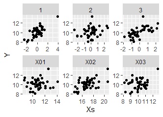
ggplot(Data_long, aes(x=Xs,y=Y)) + geom_point() + facet_wrap(~X,scales="free")#
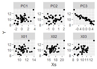
Looking at this result, we first see that there is no correlation between Y and the other variables in the original data (X01, X02, X03). Next, looking at the relationship between Y and the principal component, we can see that there is a correlation between Y and PC3. It looks like a hidden variable.
After this, we'll look at which of the original variables the hidden variable affects.
pc2 <- sweep(pc$rotation, MARGIN=2, pc$sdev, FUN="*")#
pc2#
library(heatmaply) #
heatmaply(pc2)#
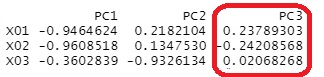
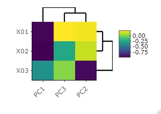
Looking at this result, it was found that the hidden variable PC3 does not seem to affect X03 because the absolute value of the factor loading is close to 0 for X03 and PC3. PC3 seems to be a factor that seems to have a slight effect on X01 and X02.
How to use Independent Component Analysis
library(fastICA) #
library(dummies) #
library(ggplot2) #
library(tidyr) #
setwd("C:/Rtest") #
Data <- read.csv("Data.csv", header=T) #
Data1 <- Data #
Y <- Data1$Y #
Data1$Y <- NULL #
Data2 <- dummy.data.frame(Data1)#
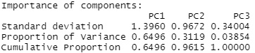
summary(prcomp(Data2, scale=TRUE))#
Data3 <- fastICA(Data2, 3)$S#
Data4 <- cbind(Y, Data2, Data3)#
Data_long <- tidyr::gather(Data4, key="X", value = Xs, -Y)#
ggplot(Data_long, aes(x=Xs,y=Y)) + geom_point() + facet_wrap(~X,scales="free")#
Looking at the relationship between Y and the independent component, it seems that there is a hidden variable because there seems to be a correlation between Y and 1.
After this, I'd like to find out which of the original variables the hidden variable affects, but I don't know how to do it like in principal component analysis. I will add it here when I understand it.
If the variable of interest is a qualitative variable
How to use principal component analysis
library(dummies) #
library(ggplot2) #
library(tidyr) #
setwd("C:/Rtest") #
Data <- read.csv("Data.csv", header=T) #
Data1 <- Data #
Y <- Data1$Y #
Data1$Y <- NULL #
Data2 <- dummy.data.frame(Data1)#
pc <- prcomp(Data2, scale=TRUE)#
Data4 <- cbind(Y, Data2, pc$x)#
Data_long <- tidyr::gather(Data4, key="X", value = Xs, -Y) #
ggplot(Data_long, aes(x=Y,y=Xs)) + geom_boxplot() + facet_wrap(~X,scales="free")#
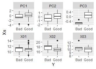
Next, looking at the relationship between Y and principal components, Y is fairly clearly separated in PC3. It looks like a hidden variable.
Finding out which of the original variables the hidden variable affects is the same as when using principal component analysis when the variable of interest is a quantitative variable.
How to use Independent Component Analysis
library(fastICA) #
library(dummies) #
library(ggplot2) #
library(tidyr) #
setwd("C:/Rtest") #
Data <- read.csv("Data.csv", header=T)#
Data1 <- Data#
Y <- Data1$Y #
Data1$Y <- NULL #
Data2 <- dummy.data.frame(Data1)#
summary(prcomp(Data2, scale=TRUE))#
Data3 <- fastICA(Data2, 3)$S#
Data4 <- cbind(Y, Data2, Data3)#
Data_long <- tidyr::gather(Data4, key="X", value = Xs, -Y) #
ggplot(Data_long, aes(x=Y,y=Xs)) + geom_boxplot() + facet_wrap(~X,scales="free")#
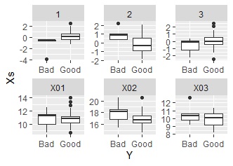
Looking at the relationship between Y and the independent component, it seems that there is a hidden variable because there seems to be a correlation between Y and 1.
