Data6 <- cbind(Data5 ,Data)Å@ #
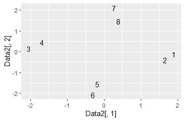
ggplot(Data6, aes(x=Data6[,1], y=Data6[,2],label=Name)) + geom_text() #

closer they are, the more similar they are. The numbers on the vertical and horizontal axes have no quantitative meaning.
The sample grouping analysis includes an explanation of what the sample grouping analysis does and an explanation of the types of methods.
At the bottom of the sample grouping analysis page, there is an explanation of "recommended method", but this page is the sample code when implementing that "recommended method" in R.
Create data to be used for MDS / t-SNE / UMAP / SOM.
Basically, we deal with quantitative variables, but since qualitative variables are coded for dummy conversion, we can mix quantitative and qualitative variables, or even just qualitative variables.
library(dummies) #
library(som) #
setwd("C:/Rtest") #
Data <- read.csv("Data.csv", header=T) #
Data1 <- Data #
Data1$Name <- NULL #
Data2 <- dummy.data.frame(Data1)#
Data3 <- normalize(Data2[,1:ncol(Data2)],byrow=F)#
Create the data to be used for the graph.
MDS, t-SNE, and SOM have advantages and disadvantages, so it seems better to use them properly.
Advantages: The easiest because there are no hyperparameters
Disadvantages: If all variables are qualitative variables, an error will occur.
library(MASS) #
Data4 <- dist(Data3)#
sn <- sammon(Data4)#
Data5 <- sn$points#
Advantages: It is easy to form a group as expected. No error occurs even if there is a combination of samples whose distance becomes 0.
Disadvantage: Even samples that do not belong to any group can be put in some group.
Smaller n_neighbors tend to cause plots to overlap. The default for n_neighbors seems to be 10, and it is easy to get an error if there are few samples. Here, "n_neighbors = 5" is set.
library(Rcpp)
library(umap)
ump_out <- umap(Data3,n_neighbors=5)
Data5 <- ump_out$layout
Advantages: All qualitative variables do not cause an error.
Disadvantage: Long calculation time. The more grids, the longer the calculation time.
library(som) #
sm <- som(Data3,xdim=10,ydim=10) #
Data5 <- sm$visual#
library(ggplot2) #
Data6 <- cbind(Data5 ,Data)Å@ #
ggplot(Data6, aes(x=Data6[,1], y=Data6[,2],label=Name)) + geom_text() #
closer they are, the more similar they are. The numbers on the vertical and horizontal axes have no quantitative meaning.
library(ggplot2) #
Data6 <- transform(Data5 ,Data,Index = row.names(Data))#
ggplot(Data6, aes(x=Data6[,1], y=Data6[,2],label=Index)) + geom_text() #
library(ggplot2) #
Data6 <- transform(Data5 ,Data, Index = row.names(Data))Å@ #
Data6$Index <- as.numeric(Data6$Index) #
ggplot(Data6, aes(x=Data6[,1], y=Data6[,2])) + geom_point(aes(colour=Index)) + scale_color_viridis_c(option = "D")#
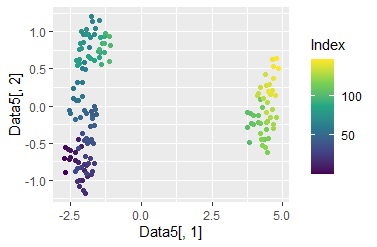
Color coded by sample number.
In the example of graph creation 3, it was found that the data is roughly divided into two areas. Therefore, I will color these two.
It's not always the color code you want, but cluster analysis makes it easy to create grouped variables.
library(ggplot2) #
library(mclust) #
mc <- Mclust(Data6[,1:2],2) #
Data7 <- transform(Data6 ,clust = mc$classification)#
Data7$clust <- as.factor(Data7$clust) #
ggplot(Data7, aes(x=Data6[,1], y=Data6[,2])) + geom_point(aes(colour=clust)) #
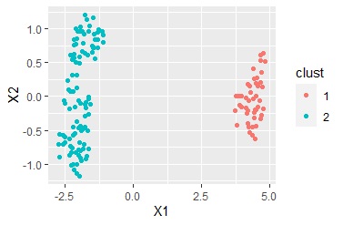
Multidimensional scaling can divide the sample into several groups, but multidimensional scaling alone does not tell you what divided it.
For the analysis after this , change the part of
Data <- read.csv("Data.csv", header=T) #
into
Data <- Data7#
and the contents of clust and others. There is a way to find out the relationship between the variables in.
In the above, the multidimensional scaling method is a flow in which the distance matrix is ??created and then the distance matrix is used as the input data of the multidimensional scaling method. So it's easy to imagine what to do if you first have the data in the form of a distance matrix.
You can start your anal
ysis with data in the form of a distance matrix using methods other than multidimensional scaling. Also, the number of dimensions of the output can be other than 2 dimensions. In the example below, it is 3 dimensions.
setwd("C:/Rtest")
Data <- read.csv("Data.csv", header=T, row.names=1)
DM <- as.matrix(Data)
library(MASS)
sn <- sammon(DM, k = 3)
Data5 <- sn$points
library(Rtsne)
ts <- Rtsne(DM, perplexity = 3, dims = 3, is_distance = TRUE)
Data5 <- ts$Y
Over 3 of dim is not available.
library(Rcpp)
library(umap)
ump_out <- umap(DM,n_neighbors=5,input='dist', n_components = 3)
Data5 <- ump_out$layout
